Chapter 6 Reproducibility and Report with R Markdown
Reproducibility is one of the core values in data science and R makes it both achievable and easy! Imagine trying to recreate someone’s analysis only to find that you get different results or that they left out crucial steps. Frustrating, right? Reproducibility is the answer—it means you can get the same results every time by following the same steps.
Why Reproducibility Matters
- Trustworthiness: When your results can be replicated, others can trust your analysis.
- Error Detection: Re-running the same code helps catch mistakes early.
- Efficiency: With reproducible scripts, you save time if you need to redo parts of your analysis.
6.1 Key Tools in R for Reproducibility and Reporting
Let’s dive into the tools that make reproducibility and reporting a breeze in R:
- R Markdown: This is the gold standard for reproducible reports in R. You can write code, comments, and format it all beautifully in one document. Think of it as combining your code with a notebook-style narrative.
- Interactive Demo: Create an R Markdown file in RStudio by clicking File > New File > R Markdown…. You can add headers, code chunks, and text.
- Run Your Code: Run each chunk individually, or click Knit to create a fully formatted report with all your code and outputs embedded.
- Setting a Seed for Consistency: R’s random number generator can be controlled with
set.seed(). For instance;
## [1] 49 65 25 74 18This will always produce the same random sample, making your analysis consistent.
- Code Commenting and Documentation: Clear comments make your analysis easy to understand for others and for yourself. Use comments (
#) in your code to describe steps, and include documentation for more complex functions.
Below is an example of a comment.
6.2 Creating Reproducible Reports
Let’s walk through a simple activity where we create a reproducible report:
- Set Up Your R Markdown File
- Open RStudio and create a new R Markdown file.
- Add a title, your name, and the date.
- Start with an introduction: Below is an example of a report to introduce R makrdown.
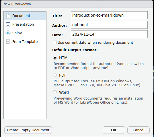
- Insert the relevant details and press Ok to create a markdown file. An introductory report explaining how markdown works will be automatically generated. For more information about R makrdown visit here
- Add Your Code and Analysis
Insert code chunks for each analysis step. For example, try loading and summarizing the mtcars data set:
##       mpg             cyl             disp             hp
##  Min.   :10.40   Min.   :4.000   Min.   : 71.1   Min.   : 52.0
##  1st Qu.:15.43   1st Qu.:4.000   1st Qu.:120.8   1st Qu.: 96.5
##  Median :19.20   Median :6.000   Median :196.3   Median :123.0
##  Mean   :20.09   Mean   :6.188   Mean   :230.7   Mean   :146.7
##  3rd Qu.:22.80   3rd Qu.:8.000   3rd Qu.:326.0   3rd Qu.:180.0
##  Max.   :33.90   Max.   :8.000   Max.   :472.0   Max.   :335.0
##       drat             wt             qsec             vs
##  Min.   :2.760   Min.   :1.513   Min.   :14.50   Min.   :0.0000
##  1st Qu.:3.080   1st Qu.:2.581   1st Qu.:16.89   1st Qu.:0.0000
##  Median :3.695   Median :3.325   Median :17.71   Median :0.0000
##  Mean   :3.597   Mean   :3.217   Mean   :17.85   Mean   :0.4375
##  3rd Qu.:3.920   3rd Qu.:3.610   3rd Qu.:18.90   3rd Qu.:1.0000
##  Max.   :4.930   Max.   :5.424   Max.   :22.90   Max.   :1.0000
##        am              gear            carb
##  Min.   :0.0000   Min.   :3.000   Min.   :1.000
##  1st Qu.:0.0000   1st Qu.:3.000   1st Qu.:2.000
##  Median :0.0000   Median :4.000   Median :2.000
##  Mean   :0.4062   Mean   :3.688   Mean   :2.812
##  3rd Qu.:1.0000   3rd Qu.:4.000   3rd Qu.:4.000
## Max. :1.0000 Max. :5.000 Max. :8.000- Customize and Style Your Report
- Add section headers, bold text, and bullet points to organize your report.
- You can use
ggplot2to add visualizations for a polished look.
library(ggplot2)
ggplot(mtcars, aes(x = hp, y = mpg)) +
  geom_point() +
  labs(title = "Horsepower vs. Miles per Gallon")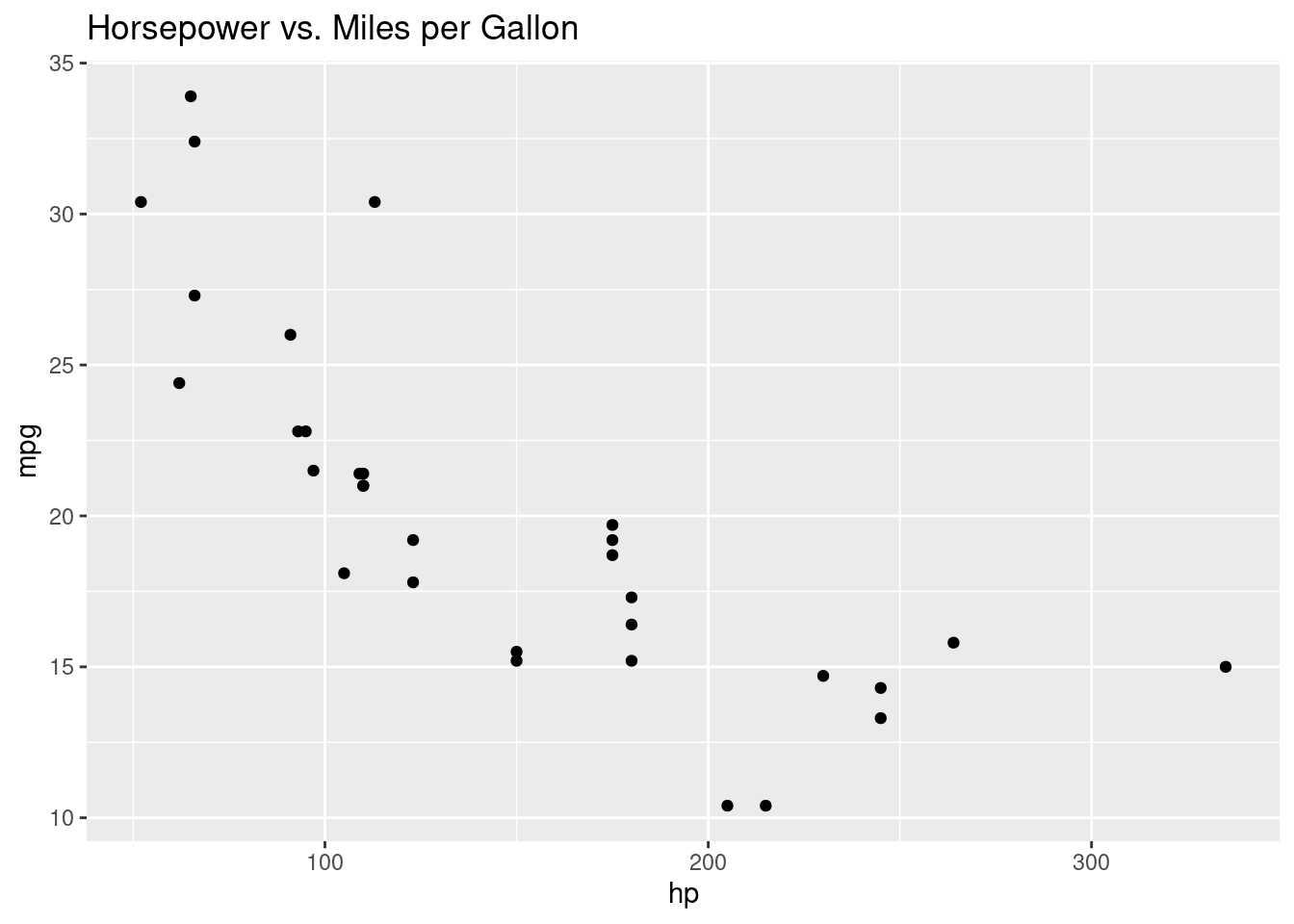
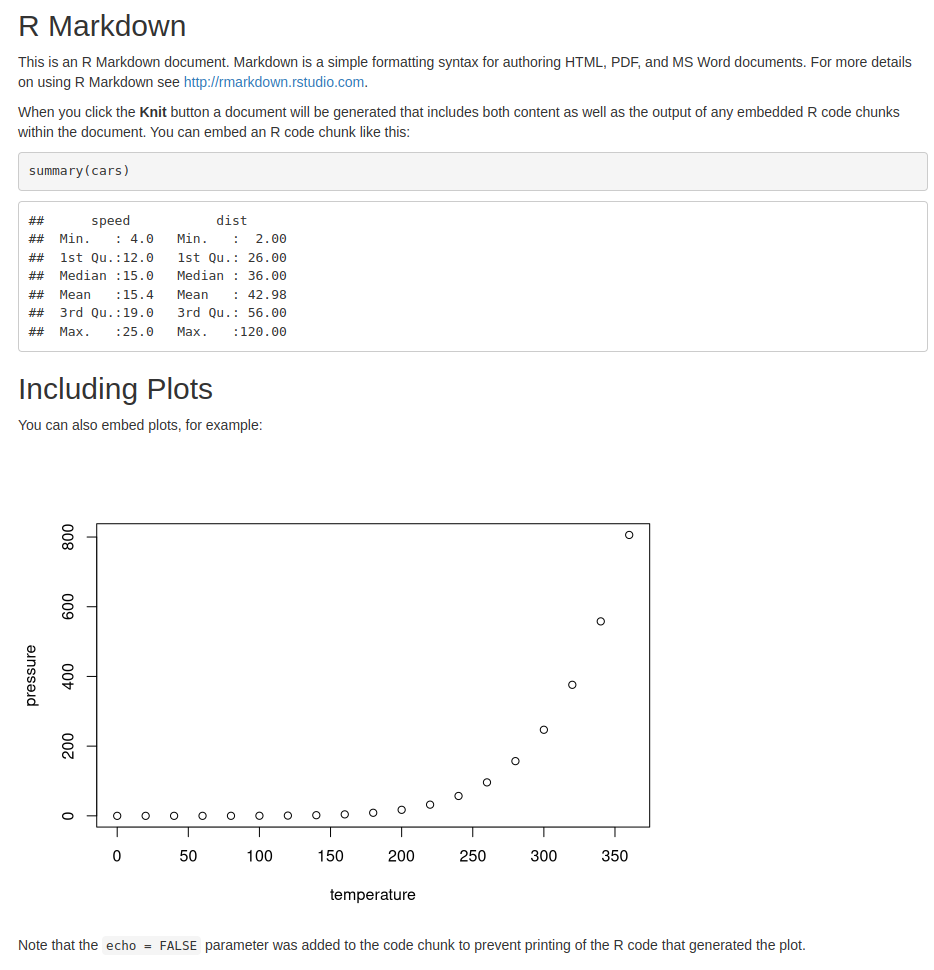
- Knit the Report
- Click the Knit button to render your report into an HTML, PDF, or Word document.
- Notice how your code, output, and comments are all integrated.
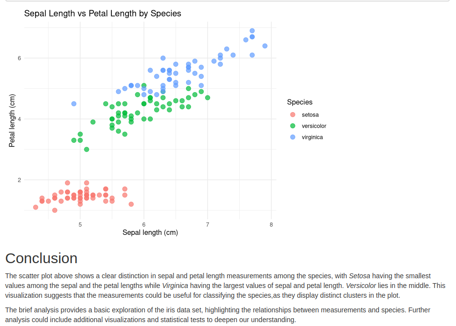
Here is how the report should look like when knitted.
6.3 Going Beyond: Shiny for Interactive Reporting
For advanced projects, consider using Shiny to create interactive reports! Shiny apps can run right in your browser and allow users to interact with your data in real time.
More details on RShiny will be discussed later on the next topic
Reproducibility is a powerful skill—keep practicing, and you’ll quickly see how it enhances your data work!
Hands-on Exercises
Create an R Markdown file with:
- A title and introduction explaining your analysis.
- An example dataset analysis (try using
irisormtcars). - A basic visualization.
- A conclusion summarizing your findings.
- Knit the report to html
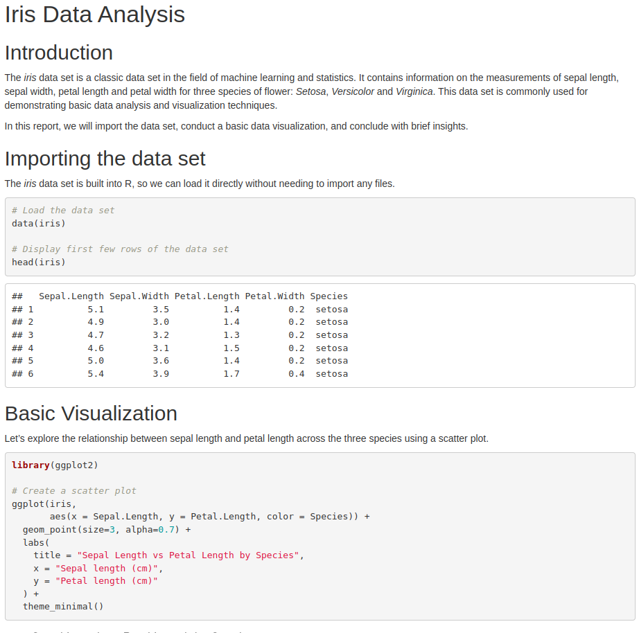
Solution
Instructor to show the students the example report(r Markdown and hmtl files) at path reproducibility_projects/example/ directory
Solution provided in reproducibility_projects/solution/solution.Rmd
Here is how the documents should look like
 ________________________________________________________________________________