Chapter 5 Simple Linear Regression

Welcome to the world of Simple Linear Regression! 🎉 This statistical technique is super handy when you want to explore the relationship between two continuous variables. Essentially, it helps us predict the value of one variable based on the value of another.

For example, imagine you want to predict a student’s exam score based on the number of hours they studied. Here, the hours studied are the independent variable (or predictor), and the exam score is the dependent variable (or response).

What is Simple Linear Regression?

Simple linear regression is essentially about finding the line that best describes the relationship between two variables(independent and dependent variables) in your data. The line is called the regression line, and it helps us make predictions.

5.1 Basics of Wilkinson-Rogers Notation (y ~ x), Linear Regression

In simple linear regression, we fit a straight line (called the regression line) through the data points. This line is defined by the equation:

\[y = mx + b\]

Where:

\(y\) is the predicted value (dependent variable).
\(m\) is the slope of the line (how much \(y\) changes for a unit change in \(x\)).
\(x\) is the independent variable.
\(b\) is the y-intercept (the value of \(y\) when \(x\) is 0).

Try it!

Lets say, we have a data set of age and height of youngsters as below here:

age = c(5, 10, 15, 20, 25)
height = c(110, 130, 150, 160, 170)

We can use the age to predict the height where age is the independent variable and height is the dependent variable(depends on age). The equation is written like this in R;

height ~ age

in short independent_variable ~ dependent_variable. Now, lets work it out using the lm() function

# Creating a sample data set
age = c(5, 10, 15, 20, 25)
height = c(110, 130, 150, 160, 170)

# Fitting a linear regression data set
model_1 <- lm(height ~ age)

The lm() function stands for ’linear model` and it finds the best line to describle the relationship between height and age.

summary(model_1)

## 
## Call:
## lm(formula = height ~ age)
## 
## Residuals:
##  1  2  3  4  5 
## -4  1  6  1 -4 
## 
## Coefficients:
##             Estimate Std. Error t value Pr(>|t|)    
## (Intercept)  99.0000     5.0662   19.54 0.000293 ***
## age           3.0000     0.3055    9.82 0.002245 ** 
## ---
## Signif. codes:  0 '***' 0.001 '**' 0.01 '*' 0.05 '.' 0.1 ' ' 1
## 
## Residual standard error: 4.83 on 3 degrees of freedom
## Multiple R-squared:  0.9698, Adjusted R-squared:  0.9598 
## F-statistic: 96.43 on 1 and 3 DF,  p-value: 0.002245

Real world challenge

Let’s use the built-in mtcars data set in R to demonstrate how to perform simple linear regression.

Load the data set

# Load the mtcars dataset
data(mtcars)
# View the first few rows of the dataset
head(mtcars)

##                    mpg cyl disp  hp drat    wt  qsec vs am gear carb
## Mazda RX4         21.0   6  160 110 3.90 2.620 16.46  0  1    4    4
## Mazda RX4 Wag     21.0   6  160 110 3.90 2.875 17.02  0  1    4    4
## Datsun 710        22.8   4  108  93 3.85 2.320 18.61  1  1    4    1
## Hornet 4 Drive    21.4   6  258 110 3.08 3.215 19.44  1  0    3    1
## Hornet Sportabout 18.7   8  360 175 3.15 3.440 17.02  0  0    3    2
## Valiant           18.1   6  225 105 2.76 3.460 20.22  1  0    3    1

Fit the simple linear regression model that will predict mpg (miles per gallon) based on wt (the weight of the car).

# Fit the linear regression model
model_2 <- lm(mpg ~ wt, data = mtcars)

Get the model summary to get important information about the model we just fitted.

# Get the summary of the model
summary(model_2)

## 
## Call:
## lm(formula = mpg ~ wt, data = mtcars)
## 
## Residuals:
##     Min      1Q  Median      3Q     Max 
## -4.5432 -2.3647 -0.1252  1.4096  6.8727 
## 
## Coefficients:
##             Estimate Std. Error t value Pr(>|t|)    
## (Intercept)  37.2851     1.8776  19.858  < 2e-16 ***
## wt           -5.3445     0.5591  -9.559 1.29e-10 ***
## ---
## Signif. codes:  0 '***' 0.001 '**' 0.01 '*' 0.05 '.' 0.1 ' ' 1
## 
## Residual standard error: 3.046 on 30 degrees of freedom
## Multiple R-squared:  0.7528, Adjusted R-squared:  0.7446 
## F-statistic: 91.38 on 1 and 30 DF,  p-value: 1.294e-10

5.2 Scatterplots with Regression Lines, Reading lm() Output

Now that we have a model in place lets plot the data and regression line to understand the relationship. You remember we have just worked on a case of where we use the age of youngsters to find their height? That’s fine! Lets plot a scatter plot and regression line to visualize the relationship between age and height.

# Scatter plot of age vs height 
plot(age, height,
     main = "Height vs Age", 
     xlab = "Age",
     ylab = "Height",pch=19,
     col = "blue"
       )

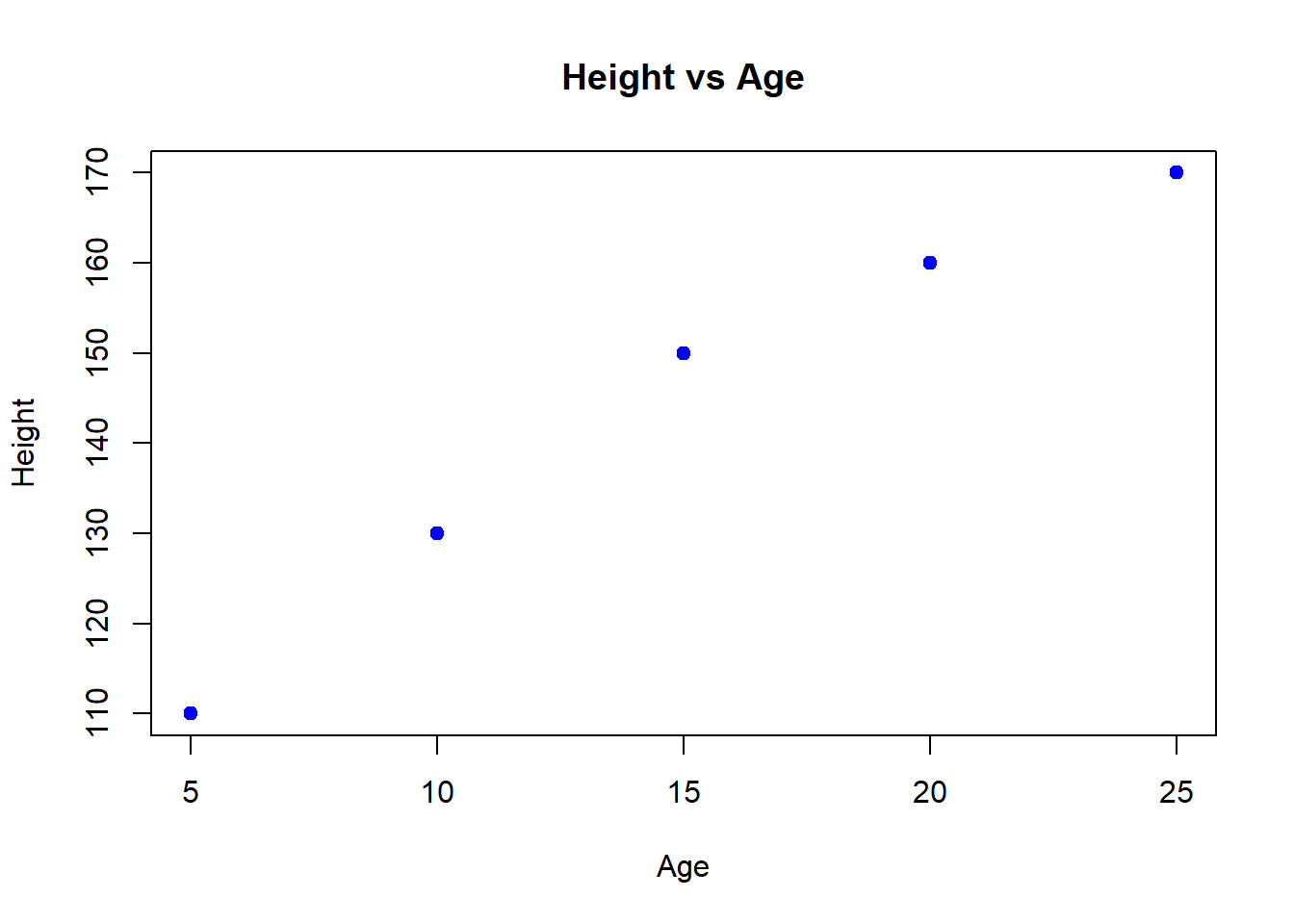
The scatter plot shows that the youngsters tend to be taller as they get older. Now lets add a regression line to the data to see how well it fits the data;

# Scatter plot of age vs height 
plot(age, height,
     main = "Height vs Age", 
     xlab = "Age",
     ylab = "Height",pch=19,
     col = "blue"
       )

# Adding a regression line 
abline(model_1, col="red", lwd=2)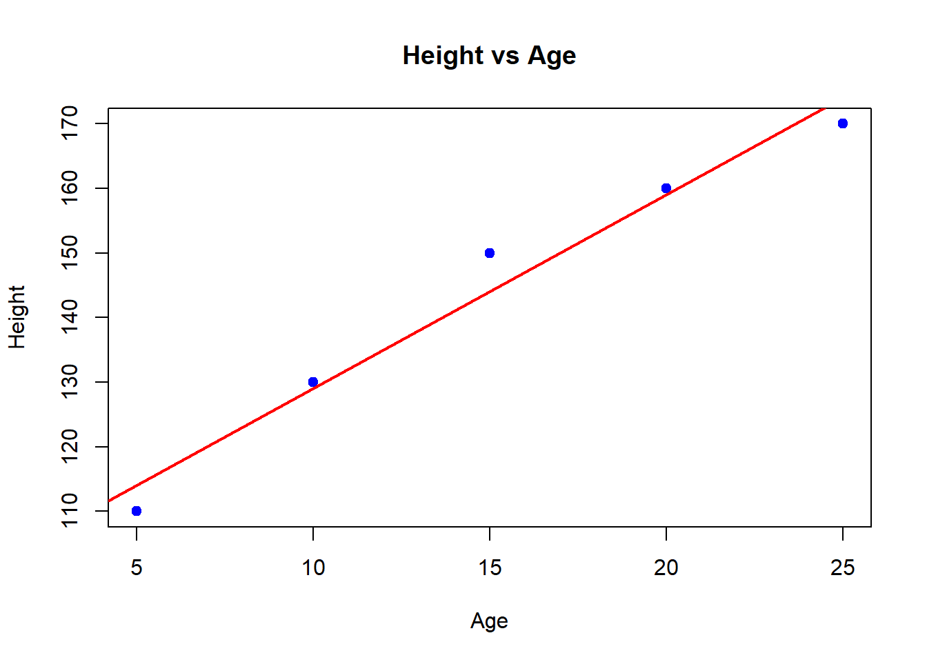

The regression line helps us visually understand the trend. In our case here, the regression line closely follows the data points, therefore, our model is a good fit!

Real World example

We will still consider the model that we created above for the mtcars data set. Lets plot a scatter plot and fit a regression line based on the model that we have just created.

# Plot the data points
plot(mtcars$wt, mtcars$mpg, 
     main = "Simple Linear Regression", 
     xlab = "Weight of the Car (wt)", 
     ylab = "Miles Per Gallon (mpg)", 
     pch = 19, col = "blue")

# Add the regression line
abline(model_2, col = "red")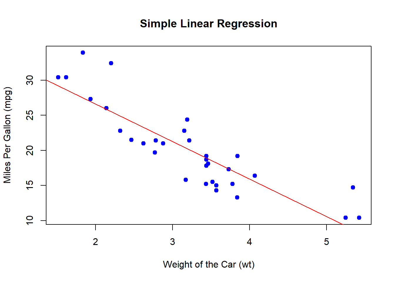

Predictions can be made based on the data. Lets predict the mpg for car that weighs 3.5 tons

# Predict mpg for a car that weighs 3.5 tons
new_data <- data.frame(wt = 3.5)
predicted_mpg <- predict(model_2, new_data)
print(paste("Predicted MPG for a car weighing 3.5 tons:", round(predicted_mpg, 2)))

## [1] "Predicted MPG for a car weighing 3.5 tons: 18.58"

5.3 Confidence Intervals for Regression Coefficients, Testing Coefficients

Lets revisit the model that we fitted age and height of youths.

summary(model_1)

## 
## Call:
## lm(formula = height ~ age)
## 
## Residuals:
##  1  2  3  4  5 
## -4  1  6  1 -4 
## 
## Coefficients:
##             Estimate Std. Error t value Pr(>|t|)    
## (Intercept)  99.0000     5.0662   19.54 0.000293 ***
## age           3.0000     0.3055    9.82 0.002245 ** 
## ---
## Signif. codes:  0 '***' 0.001 '**' 0.01 '*' 0.05 '.' 0.1 ' ' 1
## 
## Residual standard error: 4.83 on 3 degrees of freedom
## Multiple R-squared:  0.9698, Adjusted R-squared:  0.9598 
## F-statistic: 96.43 on 1 and 3 DF,  p-value: 0.002245

Here we will focus on the coefficients and the confidence intervals. The confidence interval for each regression coefficient helps us understand the range within which true value of the coeefficient is likely to fall.

The confint() function in R is used to obtain this information.

# Calculate the confidence interval 
confint(model_1)

##                 2.5 %     97.5 %
## (Intercept) 82.877001 115.122999
## age          2.027747   3.972253

As stated earlier the simple linear regression model equation is \(y = mx + b\); we will remodel this equation to fit the 2.5% and 97.5% confidence interval inform of \(height(y) = Coefficient(m) * age(x) + Intercept(b)\). Therefore:

At 2.5% confidence interval; the equation is \[height = 2.028 * age + 82.877\]
At 97.5% confidence interval; the equations is \[height = 3.972 * age + 115.123\]

Using the equations above you can estimate the height of the youth based on age.

5.4 Tests on the Regression Coefficients

In simple linear regression, we estimate a model of the form:

\[ Y = \beta_0 + \beta_1 X + \epsilon \]

where:

\(\beta_0\) (intercept) and \(\beta_1\) (slope) are the regression coefficients.
\(X\) is the independent variable.
\(Y\) is the dependent variable.
\(\epsilon\) is the random error.

5.4.1 Why Test Regression Coefficients?

To determine if the slope (\(\beta_1\)) significantly differs from zero.
To check if the intercept (\(\beta_0\)) is significant.
To assess whether the independent variable significantly predicts the dependent variable.

5.4.2 Hypothesis Testing for Regression Coefficients

The t-test is used to test the significance of the regression coefficients.

5.4.2.1 Null and Alternative Hypotheses

For the intercept (\(\beta_0\)): \[ H_0: \beta_0 = 0 \quad \text{(No significant intercept)} \] \[ H_A: \beta_0 \neq 0 \quad \text{(Intercept is significant)} \]

For the slope (\(\beta_1\)): \[ H_0: \beta_1 = 0 \quad \text{(No relationship between \(X\) and \(Y\))} \] \[ H_A: \beta_1 \neq 0 \quad \text{(Significant relationship)} \]

5.4.2.2 Example: Predicting Sales from Advertising Budget

# Load necessary library
library(ggplot2)

## Warning: package 'ggplot2' was built under R version 4.3.3

# Sample data
advertising <- c(10, 15, 20, 25, 30, 35, 40, 45, 50, 55)
sales <- c(5, 7, 8, 10, 15, 16, 18, 22, 25, 28)

# Fit the linear regression model
model <- lm(sales ~ advertising)

# Display summary
summary(model)

## 
## Call:
## lm(formula = sales ~ advertising)
## 
## Residuals:
##     Min      1Q  Median      3Q     Max 
## -1.5091 -0.8606  0.3182  0.8424  1.2727 
## 
## Coefficients:
##             Estimate Std. Error t value Pr(>|t|)    
## (Intercept) -1.46061    0.84342  -1.732    0.122    
## advertising  0.51879    0.02374  21.856 2.03e-08 ***
## ---
## Signif. codes:  0 '***' 0.001 '**' 0.01 '*' 0.05 '.' 0.1 ' ' 1
## 
## Residual standard error: 1.078 on 8 degrees of freedom
## Multiple R-squared:  0.9835, Adjusted R-squared:  0.9815 
## F-statistic: 477.7 on 1 and 8 DF,  p-value: 2.027e-08

Interpreting Regression Output

summary(model)$coefficients

##               Estimate Std. Error   t value     Pr(>|t|)
## (Intercept) -1.4606061 0.84342104 -1.731764 1.215559e-01
## advertising  0.5187879 0.02373716 21.855517 2.026551e-08

Intercept (\(\beta_0\)): Not significant (p = 0.121), meaning the model does not strongly support an inherent baseline sales value.
Slope (\(\beta_1\)): Highly significant (p = 0.00000002026551), meaning advertising budget significantly predicts sales.

5.4.3 Confidence Intervals for Regression Coefficients

We can compute confidence intervals for regression coefficients.

5.4.3.1 Example: 95% Confidence Intervals

confint(model, level = 0.95)

##                  2.5 %    97.5 %
## (Intercept) -3.4055385 0.4843263
## advertising  0.4640499 0.5735259

If the confidence interval for \(\beta_1\) does not include zero, the predictor is significant.

5.4.4 Visualizing Regression Line and Confidence Intervals

5.4.4.1 Example: Scatterplot with Regression Line

ggplot(data = data.frame(advertising, sales), aes(x = advertising, y = sales)) +
  geom_point(color = "blue") +
  geom_smooth(method = "lm", se = TRUE, color = "red") +
  labs(title = "Sales vs Advertising Budget",
       x = "Advertising Budget",
       y = "Sales") +
  theme_minimal()

## `geom_smooth()` using formula = 'y ~ x'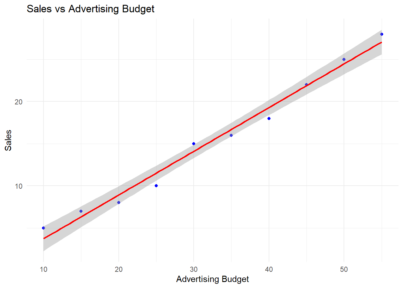

5.4.5 Testing Individual Coefficients Using `car` Package

The car package provides robust significance tests.

5.4.5.1 Example: `linearHypothesis()` for Testing \(\beta_1\)

library(car)

## Warning: package 'car' was built under R version 4.3.3

## Loading required package: carData

linearHypothesis(model, "advertising = 0")

## 
## Linear hypothesis test:
## advertising = 0
## 
## Model 1: restricted model
## Model 2: sales ~ advertising
## 
##   Res.Df   RSS Df Sum of Sq      F    Pr(>F)    
## 1      9 564.4                                  
## 2      8   9.3  1     555.1 477.66 2.027e-08 ***
## ---
## Signif. codes:  0 '***' 0.001 '**' 0.01 '*' 0.05 '.' 0.1 ' ' 1

If p-value < 0.05, we reject \(H_0\), meaning advertising has a significant effect on sales.

5.4.6 Practical Exercises

5.4.6.1 Exercise 1: Running a Regression Model

Use the dataset:

experience <- c(1, 2, 3, 4, 5, 6, 7, 8, 9, 10)
salary <- c(40000, 42000, 45000, 47000, 50000, 52000, 55000, 58000, 60000, 63000)

Fit a linear regression model predicting salary from experience.
Perform hypothesis tests on coefficients.

Solution

salary_model <- lm(salary ~ experience)
summary(salary_model)

## 
## Call:
## lm(formula = salary ~ experience)
## 
## Residuals:
##     Min      1Q  Median      3Q     Max 
## -484.85 -203.03   15.15  233.33  375.76 
## 
## Coefficients:
##             Estimate Std. Error t value Pr(>|t|)    
## (Intercept) 37066.67     219.27  169.04 1.68e-15 ***
## experience   2569.70      35.34   72.72 1.43e-12 ***
## ---
## Signif. codes:  0 '***' 0.001 '**' 0.01 '*' 0.05 '.' 0.1 ' ' 1
## 
## Residual standard error: 321 on 8 degrees of freedom
## Multiple R-squared:  0.9985, Adjusted R-squared:  0.9983 
## F-statistic:  5288 on 1 and 8 DF,  p-value: 1.425e-12

5.4.6.2 Exercise 2: Computing Confidence Intervals

Use the same dataset as Exercise 1.
Compute 95% confidence intervals for regression coefficients.

Solution

confint(salary_model, level = 0.95)

##                 2.5 %    97.5 %
## (Intercept) 36561.021 37572.312
## experience   2488.205  2651.189

5.4.6.3 Exercise 3: Testing Significance of Coefficients

Use the same dataset as Exercise 1.
Use the car package to test if experience significantly predicts salary.

Solution

library(car)
linearHypothesis(salary_model, "experience = 0")

## 
## Linear hypothesis test:
## experience = 0
## 
## Model 1: restricted model
## Model 2: salary ~ experience
## 
##   Res.Df       RSS Df Sum of Sq      F    Pr(>F)    
## 1      9 545600000                                  
## 2      8    824242  1 544775758 5287.5 1.425e-12 ***
## ---
## Signif. codes:  0 '***' 0.001 '**' 0.01 '*' 0.05 '.' 0.1 ' ' 1

5.4.6.4 Exercise 4: Visualizing Regression Model

Use the same dataset as Exercise 1.
Create a scatterplot with a regression line.

Solution

ggplot(data = data.frame(experience, salary), aes(x = experience, y = salary)) +
  geom_point(color = "blue") +
  geom_smooth(method = "lm", se = TRUE, color = "red") +
  labs(title = "Experience vs Salary",
       x = "Years of Experience",
       y = "Salary") +
  theme_minimal()

## `geom_smooth()` using formula = 'y ~ x'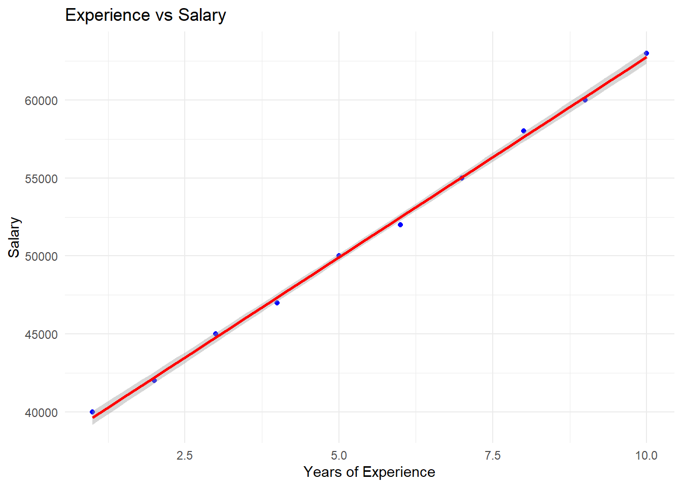

Practical Exercise

In this exercise, you will be required to use the built-in R mtcars data set. Use the weight(wt) to predict the fuel consumption(mpg). Find the equation with the confidence interval.

Solution

# Load the data 
data(mtcars)

# Fit the linear regression model
model_2 <- lm(mpg ~ wt, data = mtcars)

# Confidence intervals 
confint(model_2)

##                 2.5 %    97.5 %
## (Intercept) 33.450500 41.119753
## wt          -6.486308 -4.202635

At 2.5% confidence interval, the equation to find mpg is \[mpg = -6.486 * wt + 33.351\]
At 97.5% confidence interval, the equation to find mpg is \[mpg = -4.203 * wt + 41.120\]

________________________________________________________________________________

5.5 Identifying Points in a Plot

We made the scatter plot above static. Here, we will enable any researcher to identify specific points in the chart. I will now plot the chart using ggplot2 library.

Lets do it

library(ggplot2)

# Create the data set
height_data <- data.frame(
  age = c(5, 10, 15, 20, 25),
  height = c(110, 130, 150, 160, 170)
)

# Plot the and label the points 
ggplot(height_data, 
       aes(x = age, y = height)) + 
  geom_point(color = "blue", size=3) + # for scatter plot 
  geom_smooth(method = "lm", color="red", se = FALSE) + # regression line 
  geom_text(
    aes(label = paste("(", age, ",", height, ")", sep="")),
    vjust = -1, color = "darkgreen") + # For interactiveness 
  labs(
    title = "Age vs Height with Identified points", 
    x = "Age", 
    y = "Height"
    ) + 
  theme_classic()

## `geom_smooth()` using formula = 'y ~ x'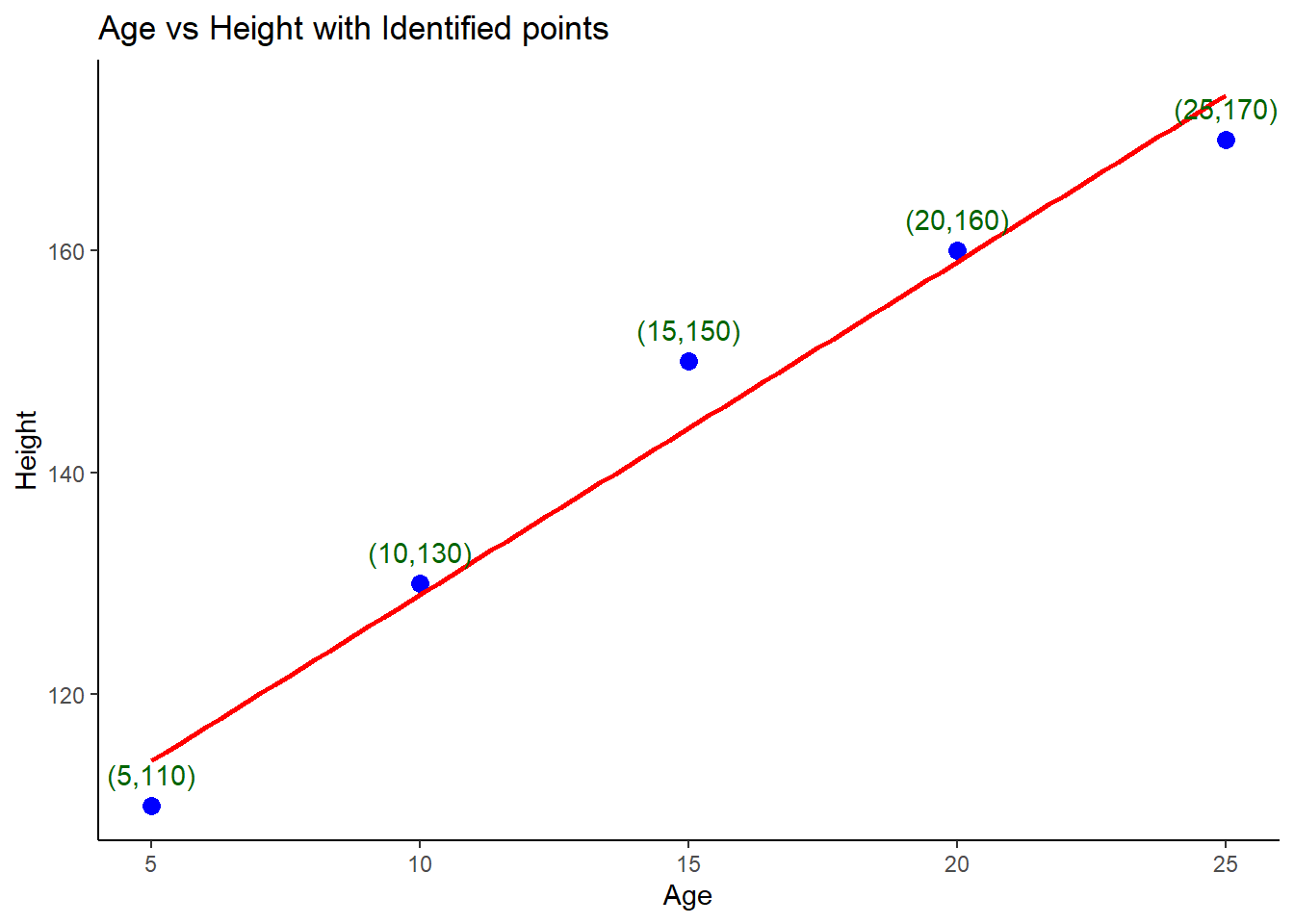

Try it!

Lets repeat the same with the mtcars data set, we will plot a weight vs fuel consumption (mpg) with identified points in the plots

library(ggplot2)

# Load the data
data(mtcars)

# Plotting
ggplot(mtcars, 
       aes(x = wt, y = mpg)) + 
  geom_point(color = "blue", size=3) + # for scatter plot 
  geom_smooth(method = "lm", color="red", se = FALSE) + # regression line 
  geom_text(
    aes(label = paste("(", wt, ",", mpg, ")", sep="")),
    vjust = -1, color = "darkgreen") + # For interactiveness 
  labs(
    title = "Wight vs mpg with Identified points", 
    x = "Weight", 
    y = "mpg"
    ) + 
  theme_classic()

## `geom_smooth()` using formula = 'y ~ x'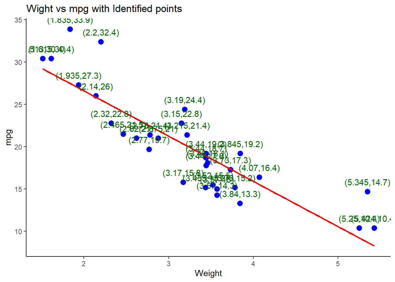

5.6 Hands-On Exercise

In this exercise, you are required to download the boston housing data set from here and answer the following questions.

Write the simple linear regression equation in form of \(y=mx + b\).
Import the data and fit the linear regression model using the lm function to find the relationship between the average number of rooms(RM) and the housing price(MEDV). MEDV is the target variable while RM is the independent variable. Generate the summary of the model
Create a scatter plot; x = RM and y = MEDV.
Add a regression line to the scatter plot.
Use the confint() function to find the coefficients at 2.5% and 97.5 confidence intervals.

Solution

Load the data and libraries

library(ggplot2)

# Import the data 
boston_housing_df <- read.csv("data/boston_housing.csv")

Write the simple linear regression equation. \[MEDV = Coefficient * RM + Intercept\]
Import the data and fit the linear regression model using the lm function to find the relationship between the average number of rooms(RM) and the housing price(MEDV). MEDV is the target variable while RM is the independent variable. Generate the summary of the model.

rm <- boston_housing_df$RM
medv <- boston_housing_df$MEDV

# Fit a linear regression model
model_3 <- lm(medv ~ rm)

# Summary of the model
summary(model_3)

## 
## Call:
## lm(formula = medv ~ rm)
## 
## Residuals:
##     Min      1Q  Median      3Q     Max 
## -23.346  -2.547   0.090   2.986  39.433 
## 
## Coefficients:
##             Estimate Std. Error t value Pr(>|t|)    
## (Intercept)  -34.671      2.650  -13.08   <2e-16 ***
## rm             9.102      0.419   21.72   <2e-16 ***
## ---
## Signif. codes:  0 '***' 0.001 '**' 0.01 '*' 0.05 '.' 0.1 ' ' 1
## 
## Residual standard error: 6.616 on 504 degrees of freedom
## Multiple R-squared:  0.4835, Adjusted R-squared:  0.4825 
## F-statistic: 471.8 on 1 and 504 DF,  p-value: < 2.2e-16

Create a scatter plot; x = RM and y = MEDV.

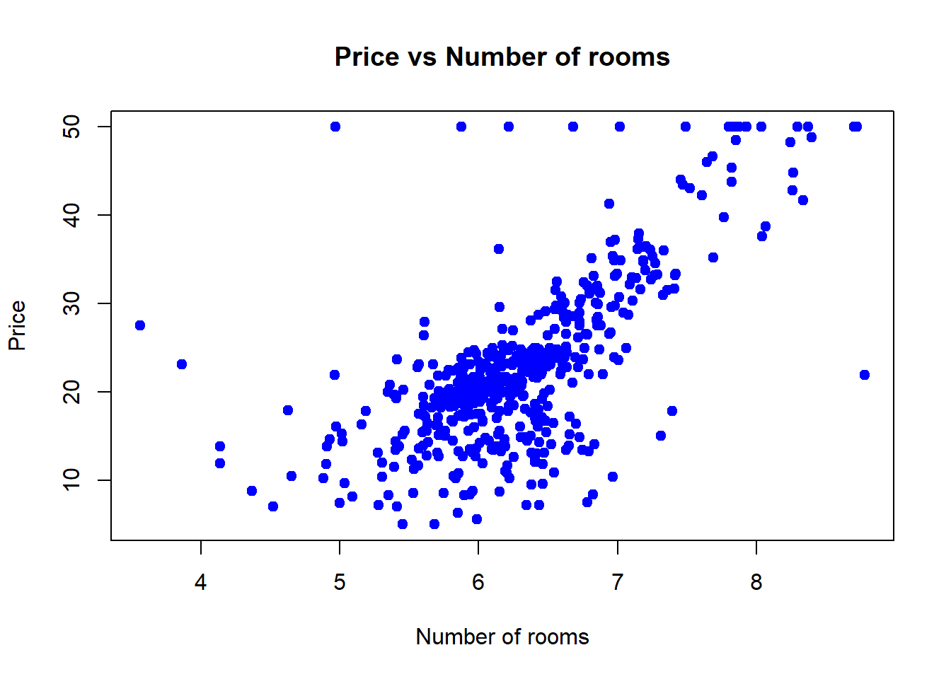
# Scatter plot of number of rooms and price
plot(rm, medv,
     main = "Price vs Number of rooms", 
     xlab = "Number of rooms",
     ylab = "Price",pch=19,
     col = "blue"
       )

Add a regression line to the scatter plot.

# Scatter plot of number of rooms and price
plot(rm, medv,
     main = "Price vs Number of rooms", 
     xlab = "Number of rooms",
     ylab = "Price",pch=19,
     col = "blue"
       )

# Add a regression line 
abline(model_3, col="red", lwd=2)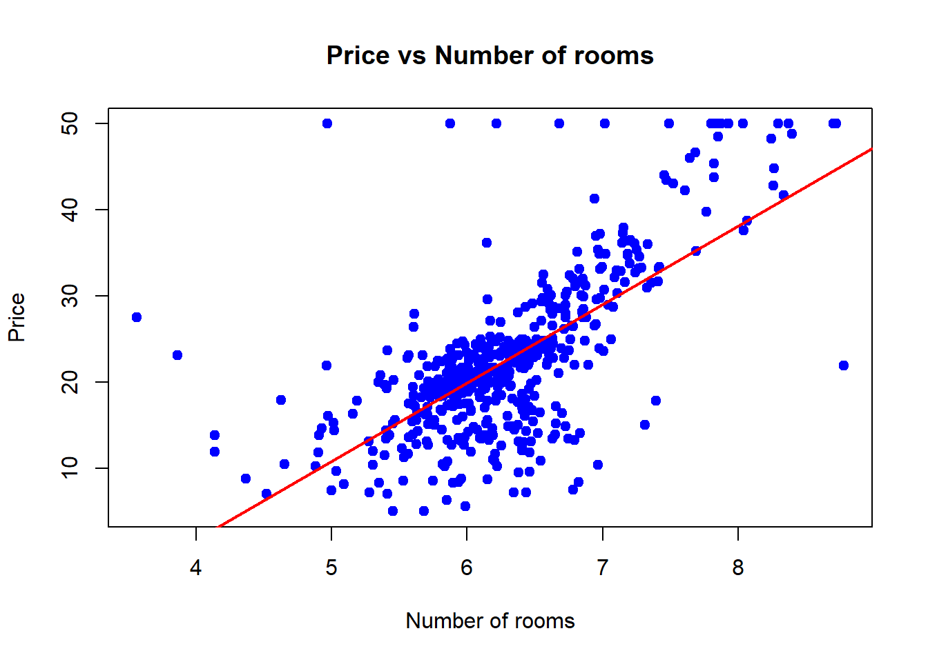

Use the confint() function to find the coefficients at 2.5% and 97.5 confidence intervals at rewrite the equations with values at each confidence interval.

confint(model_3)

##                  2.5 %     97.5 %
## (Intercept) -39.876641 -29.464601
## rm            8.278855   9.925363

At 2.5% confidence interval, the equation is \[MEDV = 8.279 * RM - 39.877\]
At 97.5 confidence level, the equation is \[MEDV = 9.925 * RM - 29.465\]

________________________________________________________________________________

Chapter 5 Simple Linear Regression

5.1 Basics of Wilkinson-Rogers Notation (y ~ x), Linear Regression

5.2 Scatterplots with Regression Lines, Reading lm() Output

5.3 Confidence Intervals for Regression Coefficients, Testing Coefficients

5.4 Tests on the Regression Coefficients

5.4.1 Why Test Regression Coefficients?

5.4.2 Hypothesis Testing for Regression Coefficients

5.4.2.1 Null and Alternative Hypotheses

5.4.2.2 Example: Predicting Sales from Advertising Budget

5.4.3 Confidence Intervals for Regression Coefficients

5.4.3.1 Example: 95% Confidence Intervals

5.4.4 Visualizing Regression Line and Confidence Intervals

5.4.4.1 Example: Scatterplot with Regression Line

5.4.5 Testing Individual Coefficients Using car Package

5.4.5.1 Example: linearHypothesis() for Testing \(\beta_1\)

5.4.6 Practical Exercises

5.4.6.1 Exercise 1: Running a Regression Model

5.4.6.2 Exercise 2: Computing Confidence Intervals

5.4.6.3 Exercise 3: Testing Significance of Coefficients

5.4.6.4 Exercise 4: Visualizing Regression Model

5.5 Identifying Points in a Plot

5.6 Hands-On Exercise

5.4.5 Testing Individual Coefficients Using `car` Package

5.4.5.1 Example: `linearHypothesis()` for Testing \(\beta_1\)