Chapter 4 General Statistics
4.1 Tabulating Factors and Creating Contingency Tables
This section explores how to handle categorical data using factors and contingency tables in R. We will learn how to:
4.1.1 Understanding Factors in R
Factors store categorical variables efficiently and allow statistical functions to recognize levels.
4.1.1.1 Example: Creating a Factor Variable
# Creating a categorical variable
survey_response <- c("Agree", "Disagree", "Neutral", "Agree", "Agree", "Disagree")

# Convert to factor
survey_factor <- factor(survey_response)

# Print the factor
print(survey_factor)
## [1] Agree Disagree Neutral Agree Agree Disagree
## Levels: Agree Disagree Neutral4.1.2 Creating Frequency Tables
A frequency table counts the number of occurrences of each category.
4.1.3 Creating Contingency Tables
A contingency table (cross-tabulation) is used to summarize two categorical variables.
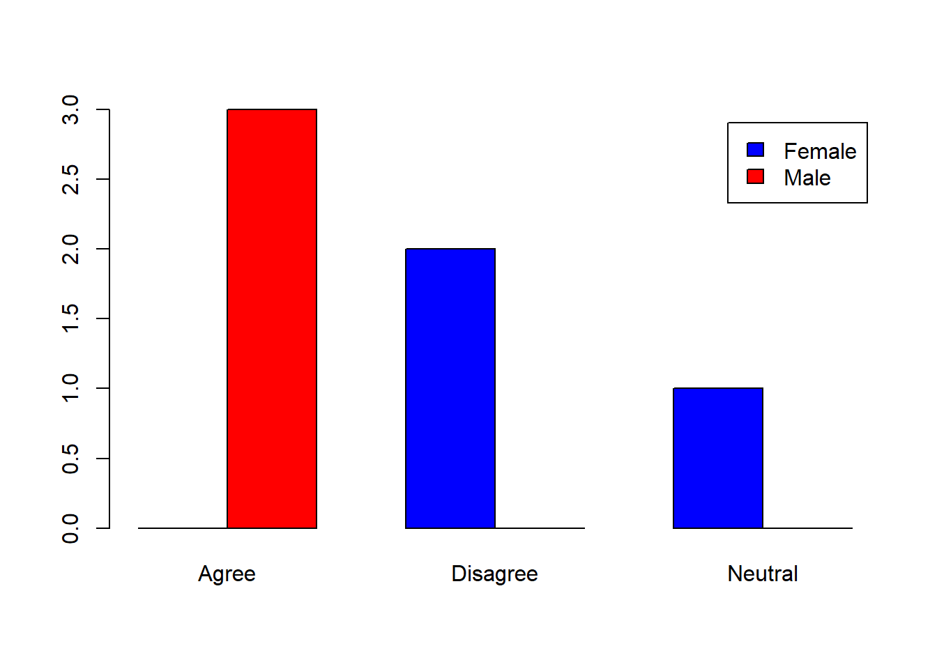
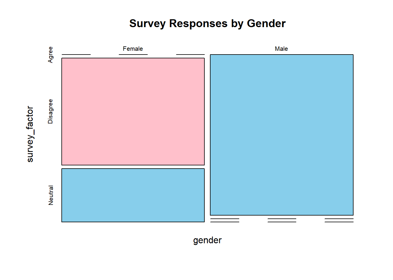
4.1.3.1 Example: 2-Way Contingency Table
# Sample data
gender <- c("Male", "Female", "Female", "Male", "Male", "Female")

# Creating a contingency table
contingency_table <- table(gender, survey_factor)

# Display the table
print(contingency_table)
## survey_factor
## gender Agree Disagree Neutral
## Female 0 2 1
## Male 3 0 04.1.5 Computing Row and Column Proportions
4.1.7 Practical Exercises
4.1.7.1 Exercise 1: Working with Factors
- Create a factor variable from the following data:
- Convert it into an ordered factor with levels:
"High School" < "College" < "Masters" < "PhD"
- Print the ordered factor.
Solution:
education_factor <- factor(education, levels = c("High School", "College", "Masters", "PhD"), ordered = TRUE)
print(education_factor)
## [1] High School College College PhD Masters High School
## Levels: High School < College < Masters < PhD4.1.7.2 Exercise 2: Creating a Contingency Table
- Create two categorical variables:
   department <- c("Sales", "HR", "IT", "Sales", "HR", "IT", "Sales", "IT")
status <- c("Full-Time", "Part-Time", "Full-Time", "Part-Time", "Full-Time", "Full-Time", "Part-Time", "Full-Time")- Generate a contingency table.
- Compute row and column proportions.
- Add margins to the table.
Solution:
# Creating a contingency table
dept_table <- table(department, status)

# Display the table
print(dept_table)
## status
## department Full-Time Part-Time
## HR 1 1
## IT 3 0
## Sales 1 2## status
## department Full-Time Part-Time
## HR 0.5000000 0.5000000
## IT 1.0000000 0.0000000
## Sales 0.3333333 0.6666667## status
## department Full-Time Part-Time
## HR 0.2000000 0.3333333
## IT 0.6000000 0.0000000
## Sales 0.2000000 0.6666667## status
## department Full-Time Part-Time Sum
## HR 1 1 2
## IT 3 0 3
## Sales 1 2 3
## Sum 5 3 84.1.7.3 Exercise 3: Titanic Dataset Analysis
Use the built-in Titanic dataset to:
Create a contingency table of passenger class (
Pclass) and survival (Survived).Compute row and column proportions.
Create a bar plot.
Solution:
# Load required packages
library(dplyr)
library(tidyr)

# Load Titanic dataset
data(Titanic)

# Convert to a proper dataframe and expand the frequency count
Titanic_df <- as.data.frame(Titanic) %>%
  uncount(Freq)  # Expands rows based on the frequency column

# Check the structure of the dataframe
str(Titanic_df)
## 'data.frame': 2201 obs. of 4 variables:
## $ Class : Factor w/ 4 levels "1st","2nd","3rd",..: 3 3 3 3 3 3 3 3 3 3 ...
## $ Sex : Factor w/ 2 levels "Male","Female": 1 1 1 1 1 1 1 1 1 1 ...
## $ Age : Factor w/ 2 levels "Child","Adult": 1 1 1 1 1 1 1 1 1 1 ...
## $ Survived: Factor w/ 2 levels "No","Yes": 1 1 1 1 1 1 1 1 1 1 ...# Create a contingency table using the correct column names
titanic_table <- table(Titanic_df$Class, Titanic_df$Survived)
# Print the table
print(titanic_table)##
## No Yes
## 1st 122 203
## 2nd 167 118
## 3rd 528 178
## Crew 673 2124.2 Calculating Quantiles
Quantiles are statistical measures that divide a dataset into equal parts. They help summarize distributions, identify outliers, and assess skewness.
4.2.1 Understanding Quantiles
Quantiles divide data into equal-sized groups:
Median (50th percentile): The middle value of a dataset.
Quartiles (25th, 50th, 75th percentiles): Divide data into four equal parts.
Deciles (10th, 20th, …, 90th percentiles): Divide data into ten equal parts.
Percentiles (1st, 2nd, …, 99th percentiles): Divide data into 100 equal parts.
4.2.4 Using summary() for Quick Insights
##    Min. 1st Qu.  Median    Mean 3rd Qu.    Max.
##    3.00    7.00   12.00   11.22   14.00   21.00
The summary() function provides:
Min: Minimum value
1st Qu. (Q1, 25%): First quartile
Median (Q2, 50%): Second quartile
Mean: Average value
3rd Qu. (Q3, 75%): Third quartile
Max: Maximum value
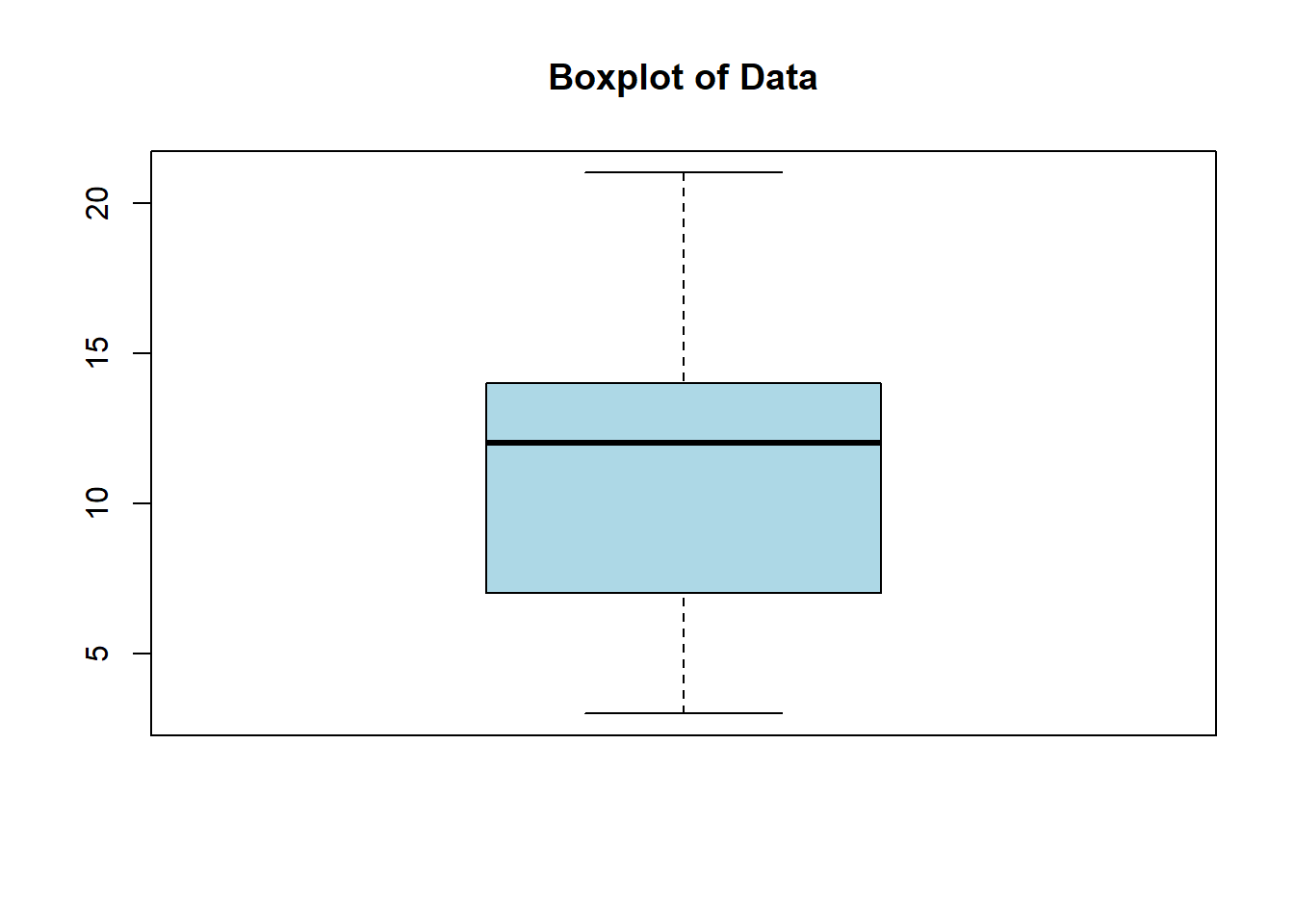 In a boxplot:
4.2.6 Finding Interquartile Range (IQR)
The IQR measures the spread of the middle 50% of the data:
## [1] 7OR manually:
## 75%
##   7
4.2.7 Finding Outliers Using IQR
Outliers are values outside Q1 - 1.5*IQR and Q3 + 1.5*IQR.
4.2.7.1 Example: Detecting Outliers
# Compute quartiles
q1 <- quantile(data, 0.25)
q3 <- quantile(data, 0.75)
iqr_value <- IQR(data)

# Define outlier thresholds
lower_bound <- q1 - 1.5 * iqr_value
upper_bound <- q3 + 1.5 * iqr_value

# Find outliers
outliers <- data[data < lower_bound | data > upper_bound]
print(outliers)
## numeric(0)4.2.8 Hands-on Exercises
4.2.8.1 Exercise 1: Computing Quartiles
- Create a dataset:
- Compute Q1, Q2 (median), and Q3.
- Calculate the IQR.
- Plot a boxplot.
Solution:
##    0%   25%   50%   75%  100%
## 55.00 74.25 83.00 89.50 95.00## [1] 15.25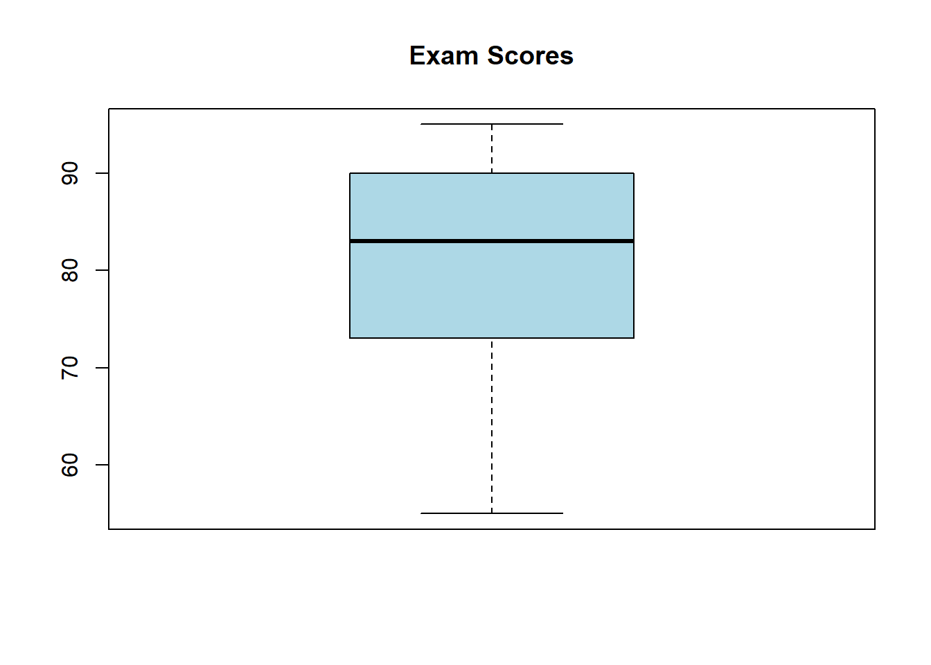
4.2.8.2 Exercise 2: Computing Custom Quantiles
- Use the dataset:
- Find the 5th, 25th, 50th, 75th, and 95th percentiles.
Solution:
##     5%    25%    50%    75%    95%
## 154.50 166.25 177.50 188.75 197.75
4.2.8.3 Exercise 3: Finding Outliers
- Use the dataset:
- Compute Q1, Q3, and IQR.
- Identify outliers.
Solution:
q1 <- quantile(salaries, 0.25)
q3 <- quantile(salaries, 0.75)
iqr_value <- IQR(salaries)

lower_bound <- q1 - 1.5 * iqr_value
upper_bound <- q3 + 1.5 * iqr_value

outliers <- salaries[salaries < lower_bound | salaries > upper_bound]
print(outliers)
## [1] 1e+054.3 z-Scores
The z-score (also called the standard score) tells us how many standard deviations a data point is from the mean. It is a useful measure for comparing values across different distributions and detecting outliers.
4.3.1 Understanding z-Scores
The z-score formula is:
\[ z = \frac{x - \mu}{\sigma} \]
Where:
\(x\) = data point
\(\mu\) = mean of the dataset
\(\sigma\) = standard deviation of the dataset
Interpretation:
\(z = 0\) → The value is equal to the mean.
\(z > 0\) → The value is above the mean.
\(z < 0\) → The value is below the mean.
\(|z| > 2\) → The value is unusual.
\(|z| > 3\) → The value is potentially an outlier.
4.3.2 Computing z-Scores in R
4.3.2.1 Example: Computing z-Scores Manually
# Sample data
data <- c(50, 55, 60, 65, 70, 75, 80, 85, 90, 95)

# Compute mean and standard deviation
mean_value <- mean(data)
sd_value <- sd(data)

# Compute z-scores
z_scores <- (data - mean_value) / sd_value
print(z_scores)
## [1] -1.4863011 -1.1560120 -0.8257228 -0.4954337 -0.1651446 0.1651446 0.4954337
## [8] 0.8257228 1.1560120 1.48630114.3.3 Computing z-Scores Using scale()
The scale() function standardizes a dataset (converts it into z-scores):
##             [,1]
##  [1,] -1.4863011
##  [2,] -1.1560120
##  [3,] -0.8257228
##  [4,] -0.4954337
##  [5,] -0.1651446
##  [6,]  0.1651446
##  [7,]  0.4954337
##  [8,]  0.8257228
##  [9,]  1.1560120
## [10,]  1.4863011
## attr(,"scaled:center")
## [1] 72.5
## attr(,"scaled:scale")
## [1] 15.13825
The scale() function automatically centers and scales the data.
4.3.4 Interpreting z-Scores
Let’s compute the z-score of 80 from our dataset:
## [1] 0.4954337If \(z = 0.5\), this means 80 is 0.5 standard deviations above the mean.
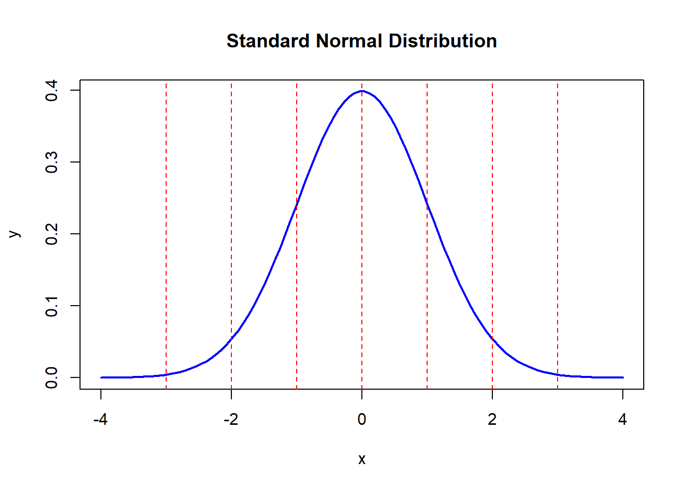
4.3.6 Visualizing z-Scores
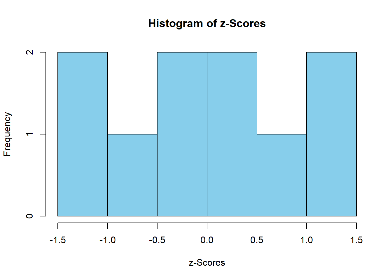
4.3.7 Hands-on Exercises
4.3.7.1 Exercise 1: Compute z-Scores
- Use the dataset:
Compute the mean and standard deviation.
Calculate the z-scores.
Find any outliers (\(|z| > 3\)).
Solution:
mean_height <- mean(heights)
sd_height <- sd(heights)
z_scores <- (heights - mean_height) / sd_height
outliers <- heights[abs(z_scores) > 3]
print(z_scores)
## [1] -1.6853070 -1.0611192 -0.7490253 -0.4369314 -0.1248376 0.1872563 0.4993502
## [8] 0.8114441 1.1235380 1.4356319## numeric(0)4.3.7.2 Exercise 2: Standardize Data Using scale()
- Use the dataset:
Standardize the data using
scale().Plot a histogram of the z-scores.
Solution:
z_weights <- scale(weights)
hist(z_weights, main = "Histogram of Standardized Weights", col = "lightgreen")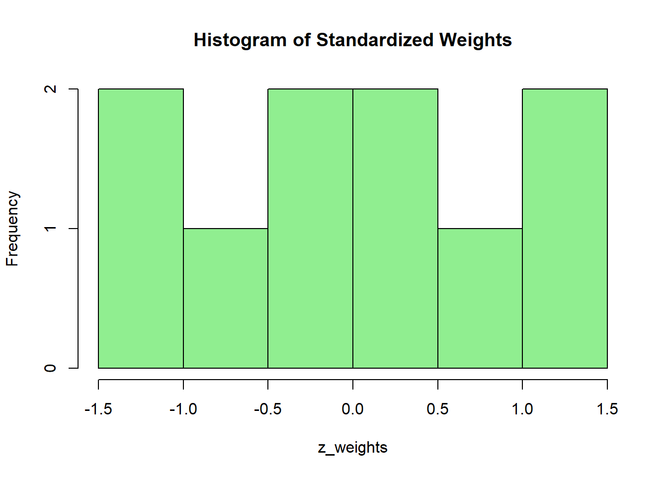
4.4 Inferential Statistics
Inferential statistics allows us to make conclusions about a population based on a sample.
4.4.1 Basic Concepts
4.4.1.1 Population vs. Sample
Population: The entire group we want to study.
Sample: A subset of the population used for analysis.
4.4.2 Confidence Intervals
A confidence interval (CI) gives a range where we expect a population parameter to lie.
4.4.2.1 Example: Confidence Interval for a Mean
# Sample data
data <- c(50, 55, 60, 65, 70, 75, 80, 85, 90, 95)

# Mean and standard deviation
mean_data <- mean(data)
sd_data <- sd(data)
n <- length(data)

# Compute confidence interval (95% confidence)
error_margin <- qt(0.975, df=n-1) * (sd_data / sqrt(n))
lower_bound <- mean_data - error_margin
upper_bound <- mean_data + error_margin

# Print confidence interval
c(lower_bound, upper_bound)
## [1] 61.67075 83.32925We are 95% confident that the population mean lies within this range.
4.4.3 Hypothesis Testing
Hypothesis testing helps us determine whether a claim about a population is supported by sample data.
4.4.4 Steps in Hypothesis Testing
State the null (\(H_0\)) and alternative (\(H_A\)) hypotheses.
Select a significance level (\(\alpha\)).
Compute the test statistic.
Compare the test statistic to a critical value or p-value.
Make a conclusion.
4.4.5 One-Sample t-Test
Tests if the sample mean is different from a known population mean.
4.4.5.1 Example: Testing If a Sample Mean Differs from 70
# Sample data
sample_data <- c(65, 68, 72, 75, 70, 66, 71, 69, 74, 67)

# One-sample t-test (H0: Mean = 70)

t.test(sample_data, mu = 70)
##
## One Sample t-test
##
## data: sample_data
## t = -0.28446, df = 9, p-value = 0.7825
## alternative hypothesis: true mean is not equal to 70
## 95 percent confidence interval:
## 67.31429 72.08571
## sample estimates:
## mean of x
## 69.7If p-value < 0.05, reject \(H_0\).
If p-value > 0.05, fail to reject \(H_0\).
4.4.6 Comparing Two Sample Means
A two-sample t-test compares the means of two independent groups.
4.4.6.1 Example: Comparing Male vs. Female Heights
# Sample data
male_heights <- c(170, 175, 180, 185, 190, 195)
female_heights <- c(160, 165, 168, 170, 175, 178)

# Two-sample t-test
t.test(male_heights, female_heights)
##
## Welch Two Sample t-test
##
## data: male_heights and female_heights
## t = 2.8225, df = 8.9621, p-value = 0.02005
## alternative hypothesis: true difference in means is not equal to 0
## 95 percent confidence interval:
## 2.607164 23.726169
## sample estimates:
## mean of x mean of y
## 182.5000 169.3333If p-value < 0.05, the means are significantly different.
If p-value > 0.05, the means are not significantly different.
4.4.7 Testing Proportions
A proportion test is used for categorical data.
4.4.7.1 Example: Testing if 60% of People Prefer Brand A
##
## 1-sample proportions test with continuity correction
##
## data: 55 out of 100, null probability 0.6
## X-squared = 0.84375, df = 1, p-value = 0.3583
## alternative hypothesis: true p is not equal to 0.6
## 95 percent confidence interval:
## 0.4475426 0.6485719
## sample estimates:
## p
## 0.55If p-value < 0.05, reject \(H_0\).
If p-value > 0.05, fail to reject \(H_0\).
4.4.8 Practical Exercises
4.4.8.1 Exercise 1: Confidence Interval for Population Mean
- Use the dataset:
- Compute a 95% confidence interval for the population mean.
Solution:
mean_weights <- mean(weights)
sd_weights <- sd(weights)
n_weights <- length(weights)
# Compute CI
error_margin <- qt(0.975, df=n_weights-1) * (sd_weights / sqrt(n_weights))
c(mean_weights - error_margin, mean_weights + error_margin)## [1] 66.67075 88.329254.4.8.2 Exercise 2: Hypothesis Test for a Mean
- Use the dataset:
- Test whether the mean test score is greater than 80.
Solution:
##
## One Sample t-test
##
## data: test_scores
## t = 3.1139, df = 9, p-value = 0.00622
## alternative hypothesis: true mean is greater than 80
## 95 percent confidence interval:
## 81.89206 Inf
## sample estimates:
## mean of x
## 84.64.4.8.3 Exercise 3: Comparing Two Sample Means
- Create two samples:
- Perform a two-sample t-test.
Solution:
##
## Welch Two Sample t-test
##
## data: group_A and group_B
## t = -0.50767, df = 12, p-value = 0.6209
## alternative hypothesis: true difference in means is not equal to 0
## 95 percent confidence interval:
## -7.559670 4.702527
## sample estimates:
## mean of x mean of y
## 22.42857 23.857144.4.8.4 Exercise 4: Testing a Sample Proportion
Suppose 45 out of 100 people prefer Product X.
Test if the true proportion is different from 50%.
Solution:
##
## 1-sample proportions test with continuity correction
##
## data: 45 out of 100, null probability 0.5
## X-squared = 0.81, df = 1, p-value = 0.3681
## alternative hypothesis: true p is not equal to 0.5
## 95 percent confidence interval:
## 0.3514281 0.5524574
## sample estimates:
## p
## 0.454.5 Testing the Mean of a Sample (t-Test) and its Confidence Interval
A t-test is used to test whether the mean of a sample is significantly different from a hypothesized population mean. It helps answer questions like:
“Is the average test score significantly different from 70?”
“Does the sample data suggest a real effect, or is it due to random chance?”
4.5.1 Understanding the t-Test
The one-sample t-test formula:
\[ t = \frac{\bar{x} - \mu}{s / \sqrt{n}} \]
Where:
\(\bar{x}\) = sample mean
\(\mu\) = population mean
\(s\) = sample standard deviation
\(n\) = sample size
4.5.2 Computing Confidence Intervals for the Mean
A confidence interval (CI) provides a range where the true population mean is expected to lie.
4.5.2.1 Example: 95% Confidence Interval for a Sample Mean
# Sample data
data <- c(55, 60, 65, 70, 75, 80, 85, 90, 95, 100)
# Compute mean, standard deviation, and sample size
mean_data <- mean(data)
sd_data <- sd(data)
n <- length(data)
# Compute confidence interval (95% confidence level)
error_margin <- qt(0.975, df=n-1) * (sd_data / sqrt(n))
lower_bound <- mean_data - error_margin
upper_bound <- mean_data + error_margin
# Print confidence interval
c(lower_bound, upper_bound)## [1] 66.67075 88.32925We are 95% confident that the population mean lies within this range.
4.5.3 Performing a One-Sample t-Test
A one-sample t-test checks whether the sample mean is significantly different from a given value.
4.5.3.1 Example: Testing if the Mean is Different from 70
# Sample data
sample_data <- c(65, 68, 72, 75, 70, 66, 71, 69, 74, 67)
# Perform one-sample t-test
t.test(sample_data, mu = 70)##
## One Sample t-test
##
## data: sample_data
## t = -0.28446, df = 9, p-value = 0.7825
## alternative hypothesis: true mean is not equal to 70
## 95 percent confidence interval:
## 67.31429 72.08571
## sample estimates:
## mean of x
## 69.7If p-value < 0.05, reject \(H_0\) → The mean is significantly different from 70.
If p-value > 0.05, fail to reject \(H_0\) → No significant difference.
4.5.4 One-Sided vs. Two-Sided Tests
By default, t.test() performs a two-sided test (\(H_A: \mu \neq 70\)).
If we want to test whether the mean is greater than or less than a value:
4.5.4.1 Example: Testing if Mean is Greater Than 70
##
## One Sample t-test
##
## data: sample_data
## t = -0.28446, df = 9, p-value = 0.6088
## alternative hypothesis: true mean is greater than 70
## 95 percent confidence interval:
## 67.76676 Inf
## sample estimates:
## mean of x
## 69.74.5.5 Comparing Two Sample Means (Independent t-Test)
A two-sample t-test checks if two groups have significantly different means.
4.5.5.1 Example: Comparing Male vs. Female Heights
# Sample data
male_heights <- c(170, 175, 180, 185, 190, 195)
female_heights <- c(160, 165, 168, 170, 175, 178)
# Perform independent t-test
t.test(male_heights, female_heights)##
## Welch Two Sample t-test
##
## data: male_heights and female_heights
## t = 2.8225, df = 8.9621, p-value = 0.02005
## alternative hypothesis: true difference in means is not equal to 0
## 95 percent confidence interval:
## 2.607164 23.726169
## sample estimates:
## mean of x mean of y
## 182.5000 169.33334.5.6 Paired t-Test (Dependent Samples)
A paired t-test compares before and after measurements.
4.5.6.1 Example: Testing Before vs. After Training Scores
# Scores before and after training
before <- c(60, 65, 70, 75, 80, 85, 90)
after <- c(65, 68, 75, 78, 85, 88, 92)
# Perform paired t-test
t.test(before, after, paired = TRUE)##
## Paired t-test
##
## data: before and after
## t = -7.8393, df = 6, p-value = 0.0002277
## alternative hypothesis: true mean difference is not equal to 0
## 95 percent confidence interval:
## -4.873641 -2.554930
## sample estimates:
## mean difference
## -3.7142864.5.7 Practical Exercises
4.5.7.1 Exercise 1: Compute a Confidence Interval
- Use the dataset:
- Compute a 95% confidence interval for the mean.
Solution:
mean_scores <- mean(scores)
sd_scores <- sd(scores)
n_scores <- length(scores)
# Compute CI
error_margin <- qt(0.975, df=n_scores-1) * (sd_scores / sqrt(n_scores))
c(mean_scores - error_margin, mean_scores + error_margin)## [1] 81.25826 87.941744.5.7.2 Exercise 2: One-Sample t-Test
- Use the dataset:
- Test whether the mean is different from 72.
Solution:
##
## One Sample t-test
##
## data: weights
## t = 1.1489, df = 9, p-value = 0.2802
## alternative hypothesis: true mean is not equal to 72
## 95 percent confidence interval:
## 66.67075 88.32925
## sample estimates:
## mean of x
## 77.54.5.7.3 Exercise 3: Comparing Two Groups
- Use the dataset:
- Perform an independent two-sample t-test.
Solution:
##
## Welch Two Sample t-test
##
## data: group_A and group_B
## t = -0.50767, df = 12, p-value = 0.6209
## alternative hypothesis: true difference in means is not equal to 0
## 95 percent confidence interval:
## -7.559670 4.702527
## sample estimates:
## mean of x mean of y
## 22.42857 23.857144.5.7.4 Exercise 4: Paired t-Test
- A study measures reaction time before and after caffeine consumption:
before_caffeine <- c(300, 320, 310, 305, 315, 290, 295)
after_caffeine <- c(280, 300, 290, 285, 295, 275, 280)- Perform a paired t-test to determine if caffeine affects reaction time.
Solution:
##
## Paired t-test
##
## data: before_caffeine and after_caffeine
## t = 20.14, df = 6, p-value = 9.733e-07
## alternative hypothesis: true mean difference is not equal to 0
## 95 percent confidence interval:
## 16.31504 20.82782
## sample estimates:
## mean difference
## 18.571434.6 Testing a Sample Proportion and its Confidence Interval
A proportion test is used when we want to make inferences about categorical data. This test helps us:
Estimate the proportion of a population with a certain characteristic.
Determine whether a sample proportion differs significantly from a hypothesized value.
4.6.1 Understanding Proportion Testing
A sample proportion is calculated as:
\[ \hat{p} = \frac{x}{n} \]
Where:
\(x\) = Number of successes (e.g., people who answered “Yes”)
\(n\) = Total number of observations
The confidence interval (CI) for a proportion is given by:
\[ \hat{p} \pm Z \times \sqrt{\frac{\hat{p}(1 - \hat{p})}{n}} \]
Where:
\(Z\) = Critical value for the confidence level (e.g., 1.96 for 95%)
\(\hat{p}\) = Sample proportion
\(n\) = Sample size
4.6.2 Computing Confidence Intervals for Proportions
We can calculate confidence intervals for proportions using prop.test().
4.6.2.1 Example: 95% Confidence Interval for Proportion
Suppose 60 out of 100 people prefer Brand A.
# Number of successes (people preferring Brand A)
x <- 60
# Total sample size
n <- 100
# Compute confidence interval
prop.test(x, n, conf.level = 0.95, correct = FALSE)##
## 1-sample proportions test without continuity correction
##
## data: x out of n, null probability 0.5
## X-squared = 4, df = 1, p-value = 0.0455
## alternative hypothesis: true p is not equal to 0.5
## 95 percent confidence interval:
## 0.5020026 0.6905987
## sample estimates:
## p
## 0.6We are 95% confident that the true proportion of people who prefer Brand A falls within the computed confidence interval.
4.6.3 Performing a One-Sample Proportion Test
We test whether a sample proportion is significantly different from a hypothesized proportion \(p_0\).
4.6.3.1 Example: Testing if 60% Prefer Brand A
We test:
\[ H_0: p = 0.60 \]
\[ H_A: p \neq 0.60 \]
##
## 1-sample proportions test without continuity correction
##
## data: x out of n, null probability 0.6
## X-squared = 0, df = 1, p-value = 1
## alternative hypothesis: true p is not equal to 0.6
## 95 percent confidence interval:
## 0.5020026 0.6905987
## sample estimates:
## p
## 0.6If p-value < 0.05, reject \(H_0\) → The sample proportion is significantly different from 60%.
If p-value > 0.05, fail to reject \(H_0\) → No significant difference.
4.6.4 One-Sided Proportion Tests
If we want to test if the proportion is greater than or less than a given value:
4.6.4.1 Example: Testing if Proportion is Greater Than 50%
##
## 1-sample proportions test without continuity correction
##
## data: x out of n, null probability 0.5
## X-squared = 4, df = 1, p-value = 0.02275
## alternative hypothesis: true p is greater than 0.5
## 95 percent confidence interval:
## 0.5178095 1.0000000
## sample estimates:
## p
## 0.64.6.4.2 Example: Testing if Proportion is Less Than 70%
##
## 1-sample proportions test without continuity correction
##
## data: x out of n, null probability 0.7
## X-squared = 4.7619, df = 1, p-value = 0.01455
## alternative hypothesis: true p is less than 0.7
## 95 percent confidence interval:
## 0.0000000 0.6769219
## sample estimates:
## p
## 0.64.6.5 Comparing Two Sample Proportions
We can compare two proportions to determine if they are significantly different.
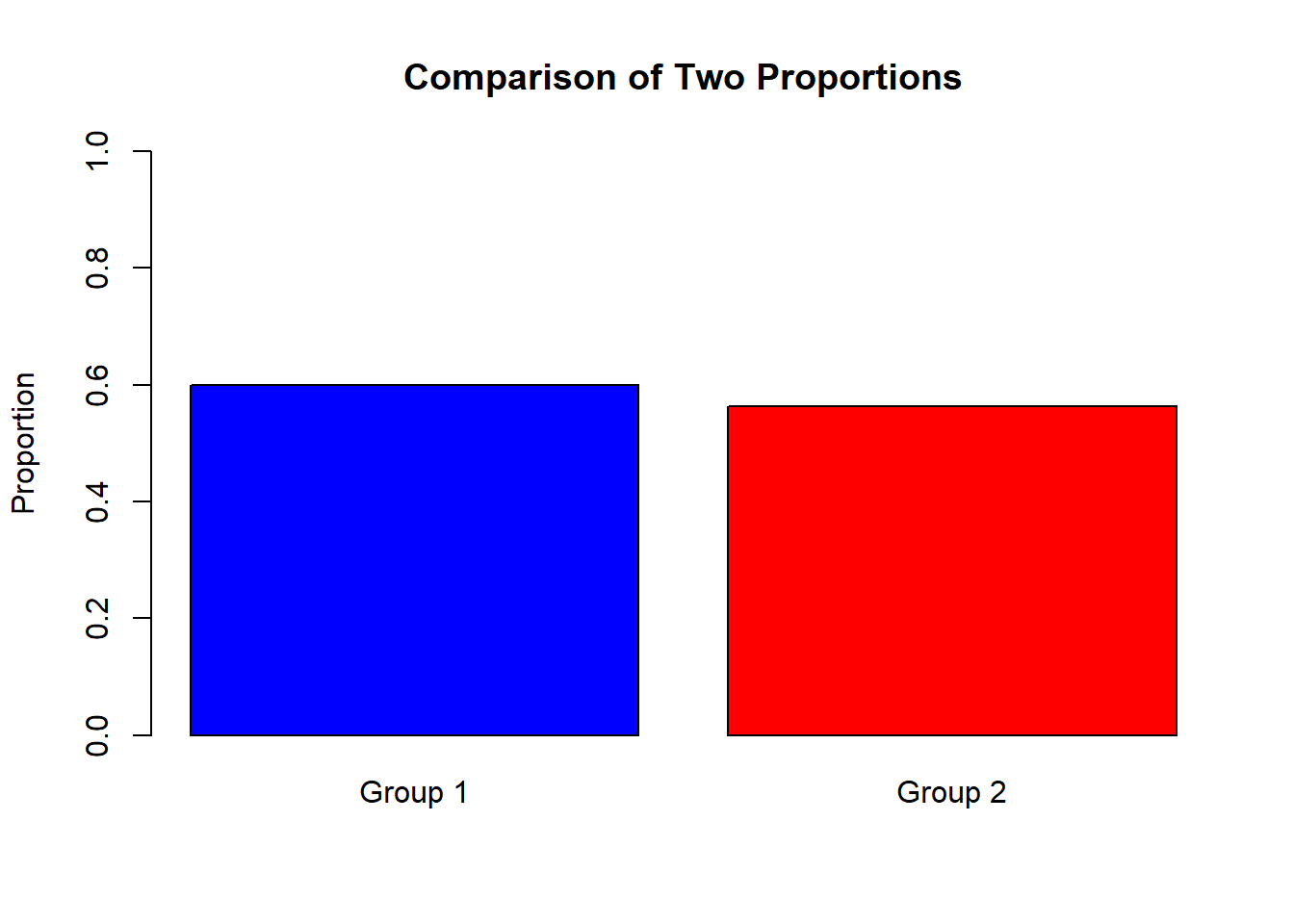
4.6.5.1 Example: Comparing Success Rates of Two Groups
Group 1: 30 successes out of 50
Group 2: 45 successes out of 80
##
## 2-sample test for equality of proportions without continuity correction
##
## data: c(30, 45) out of c(50, 80)
## X-squared = 0.17727, df = 1, p-value = 0.6737
## alternative hypothesis: two.sided
## 95 percent confidence interval:
## -0.1364425 0.2114425
## sample estimates:
## prop 1 prop 2
## 0.6000 0.5625If p-value < 0.05, the two proportions are significantly different.
If p-value > 0.05, no significant difference.
4.6.7 Practical Exercises
4.6.7.1 Exercise 1: Compute a Confidence Interval
A survey shows that 150 out of 500 people support a new policy.
Compute a 95% confidence interval for the proportion.
Solution:
##
## 1-sample proportions test without continuity correction
##
## data: 150 out of 500, null probability 0.5
## X-squared = 80, df = 1, p-value < 2.2e-16
## alternative hypothesis: true p is not equal to 0.5
## 95 percent confidence interval:
## 0.2614819 0.3415678
## sample estimates:
## p
## 0.34.6.7.2 Exercise 2: One-Sample Proportion Test
A sample of 200 students finds that 140 prefer online learning.
Test if the proportion is different from 65%.
Solution:
##
## 1-sample proportions test without continuity correction
##
## data: 140 out of 200, null probability 0.65
## X-squared = 2.1978, df = 1, p-value = 0.1382
## alternative hypothesis: true p is not equal to 0.65
## 95 percent confidence interval:
## 0.6332093 0.7592526
## sample estimates:
## p
## 0.74.6.7.3 Exercise 3: One-Sided Proportion Test
In a company, 45 out of 100 employees prefer remote work.
Test if the proportion is greater than 40%.
Solution:
##
## 1-sample proportions test without continuity correction
##
## data: 45 out of 100, null probability 0.4
## X-squared = 1.0417, df = 1, p-value = 0.1537
## alternative hypothesis: true p is greater than 0.4
## 95 percent confidence interval:
## 0.370561 1.000000
## sample estimates:
## p
## 0.454.6.7.4 Exercise 4: Comparing Two Proportions
- Two groups were surveyed:
Group A: 85 out of 150 prefer a new product.
Group B: 75 out of 130 prefer the new product.
- Test whether the proportions are significantly different.
Solution:
##
## 2-sample test for equality of proportions without continuity correction
##
## data: c(85, 75) out of c(150, 130)
## X-squared = 0.029915, df = 1, p-value = 0.8627
## alternative hypothesis: two.sided
## 95 percent confidence interval:
## -0.1264510 0.1059382
## sample estimates:
## prop 1 prop 2
## 0.5666667 0.57692314.7 Comparing the Means of Two Samples
Comparing the means of two independent samples is essential in determining if there is a significant difference between two groups.
4.7.1 Understanding Two-Sample t-Test
The two-sample t-test checks whether the means of two independent groups are significantly different.
Hypotheses:
Null Hypothesis (\(H_0\)): The two group means are equal.
Alternative Hypothesis (\(H_A\)): The two group means are different.
\[ t = \frac{\bar{x_1} - \bar{x_2}}{\sqrt{\frac{s_1^2}{n_1} + \frac{s_2^2}{n_2}}} \]
Where:
\(\bar{x_1}, \bar{x_2}\) = Sample means
\(s_1, s_2\) = Standard deviations
\(n_1, n_2\) = Sample sizes
4.7.2 Independent (Unpaired) t-Test
This test is used when the two samples are independent.
4.7.2.1 Example: Comparing Heights of Males and Females
# Sample data
male_heights <- c(170, 175, 180, 185, 190, 195)
female_heights <- c(160, 165, 168, 170, 175, 178)
# Perform independent t-test
t.test(male_heights, female_heights)##
## Welch Two Sample t-test
##
## data: male_heights and female_heights
## t = 2.8225, df = 8.9621, p-value = 0.02005
## alternative hypothesis: true difference in means is not equal to 0
## 95 percent confidence interval:
## 2.607164 23.726169
## sample estimates:
## mean of x mean of y
## 182.5000 169.3333If p-value < 0.05, reject \(H_0\) → The two means are significantly different.
If p-value > 0.05, fail to reject \(H_0\) → No significant difference.
4.7.3 Checking Assumptions
Before running a t-test, we must check:
Normality (Use Shapiro-Wilk test)
Equal Variances (Use F-test)
4.7.3.1 Example: Checking Normality
##
## Shapiro-Wilk normality test
##
## data: male_heights
## W = 0.98189, p-value = 0.9606##
## Shapiro-Wilk normality test
##
## data: female_heights
## W = 0.9841, p-value = 0.974.7.3.2 Example: Checking Equal Variances
##
## F test to compare two variances
##
## data: male_heights and female_heights
## F = 2.0317, num df = 5, denom df = 5, p-value = 0.4551
## alternative hypothesis: true ratio of variances is not equal to 1
## 95 percent confidence interval:
## 0.2843024 14.5195451
## sample estimates:
## ratio of variances
## 2.031734If p-value < 0.05, variances are not equal → Use
var.equal = FALSEint.test().If p-value > 0.05, variances are equal → Use
var.equal = TRUE.
4.7.4 Performing t-Test with Unequal Variances
4.7.4.1 Example: When Variances are Unequal
##
##  Welch Two Sample t-test
##
## data:  male_heights and female_heights
## t = 2.8225, df = 8.9621, p-value = 0.02005
## alternative hypothesis: true difference in means is not equal to 0
## 95 percent confidence interval:
##   2.607164 23.726169
## sample estimates:
## mean of x mean of y
## 182.5000 169.33334.7.4.2 Example: When Variances are Equal
##
## Two Sample t-test
##
## data: male_heights and female_heights
## t = 2.8225, df = 10, p-value = 0.01808
## alternative hypothesis: true difference in means is not equal to 0
## 95 percent confidence interval:
## 2.772665 23.560668
## sample estimates:
## mean of x mean of y
## 182.5000 169.33334.7.5 Paired t-Test (Dependent Samples)
A paired t-test is used when the same subjects are measured twice (e.g., before and after treatment).
4.7.5.1 Example: Testing Before vs. After Training Scores
# Scores before and after training
before <- c(60, 65, 70, 75, 80, 85, 90)
after  <- c(65, 68, 75, 78, 85, 88, 92)

# Perform paired t-test
t.test(before, after, paired = TRUE)
##
## Paired t-test
##
## data: before and after
## t = -7.8393, df = 6, p-value = 0.0002277
## alternative hypothesis: true mean difference is not equal to 0
## 95 percent confidence interval:
## -4.873641 -2.554930
## sample estimates:
## mean difference
## -3.714286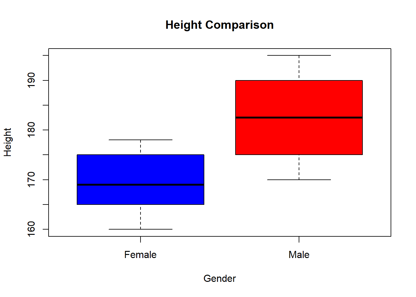
4.7.7 Practical Exercises
4.7.7.1 Exercise 1: Independent t-Test
- Two groups take an exam:
- Test if their mean scores are significantly different.
Solution:
##
## Welch Two Sample t-test
##
## data: group_A and group_B
## t = 0.92929, df = 11.951, p-value = 0.3711
## alternative hypothesis: true difference in means is not equal to 0
## 95 percent confidence interval:
## -4.037004 10.037004
## sample estimates:
## mean of x mean of y
## 86.85714 83.857144.7.7.2 Exercise 2: Checking Assumptions
- Use the dataset:
- Check for normality and equal variances.
Solution:
##
## Shapiro-Wilk normality test
##
## data: data_1
## W = 0.98189, p-value = 0.9606##
## Shapiro-Wilk normality test
##
## data: data_2
## W = 0.94009, p-value = 0.6599##
## F test to compare two variances
##
## data: data_1 and data_2
## F = 1.7797, num df = 5, denom df = 5, p-value = 0.5423
## alternative hypothesis: true ratio of variances is not equal to 1
## 95 percent confidence interval:
## 0.2490297 12.7181372
## sample estimates:
## ratio of variances
## 1.7796614.7.7.3 Exercise 3: Paired t-Test
- A fitness test is conducted before and after training:
- Test if there is a significant improvement after training.
Solution:
##
## Paired t-test
##
## data: before_fitness and after_fitness
## t = -11.5, df = 6, p-value = 2.597e-05
## alternative hypothesis: true mean difference is not equal to 0
## 95 percent confidence interval:
## -3.984832 -2.586597
## sample estimates:
## mean difference
## -3.2857144.7.8 Exercise 4: Visualizing Group Differences
- Create two datasets:
- Plot a boxplot to compare the groups.
Solution:
# Combine data into dataframe
data <- data.frame(
Score = c(treatment, control),
Group = rep(c("Treatment", "Control"), each = 5)
)
# Plot boxplot
boxplot(Score ~ Group, data = data, col = c("blue", "red"), main = "Treatment vs. Control")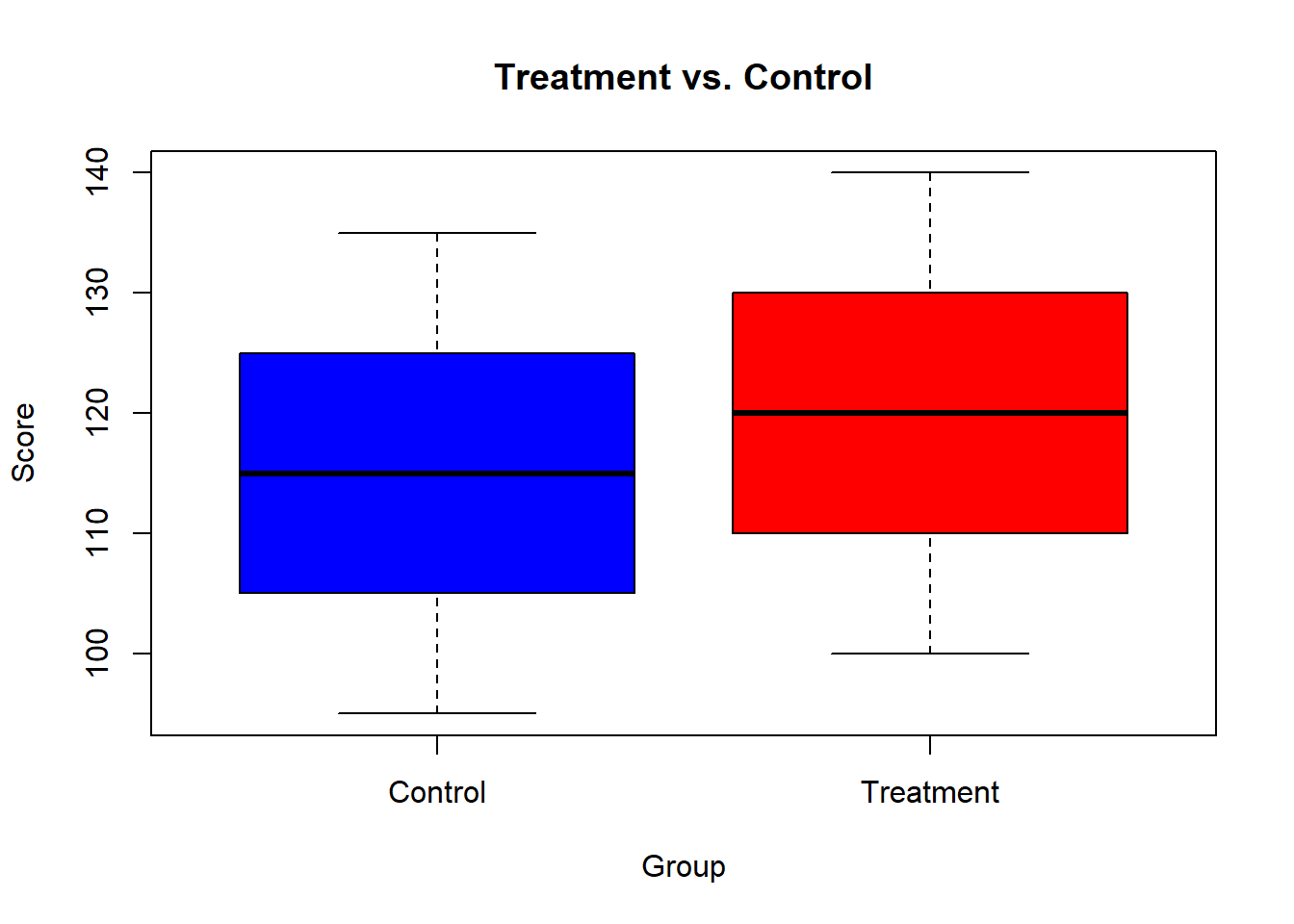
4.8 Performing Pairwise Comparisons Between Group Means
When comparing more than two groups, pairwise comparisons allow us to identify which groups differ significantly.
Common methods include:
t-Tests with adjustments for multiple comparisons
Tukey’s Honest Significant Difference (HSD) test
Bonferroni correction
Dunnett’s test (comparing to a control group)
4.8.1 Understanding Pairwise Comparisons
When comparing multiple groups, running multiple t-tests increases the risk of Type I errors (false positives).
To correct this, we apply multiple comparison adjustments like:
Bonferroni correction (divides alpha by the number of comparisons)
Holm correction (stepwise adjustment)
Tukey’s HSD (for ANOVA post-hoc comparisons)
4.8.2 Performing Pairwise t-Tests
The pairwise.t.test() function performs multiple t-tests while adjusting for multiple comparisons.
4.8.2.1 Example: Comparing Exam Scores Across Three Groups
# Sample data
group <- rep(c("Group A", "Group B", "Group C"), each = 5)
scores <- c(85, 88, 90, 92, 94, 78, 80, 83, 85, 87, 70, 72, 75, 77, 79)
### Perform pairwise t-tests with Bonferroni correction
pairwise.t.test(scores, group, p.adjust.method = "bonferroni")##
## Pairwise comparisons using t tests with pooled SD
##
## data: scores and group
##
## Group A Group B
## Group B 0.024 -
## Group C 6.8e-05 0.013
##
## P value adjustment method: bonferroniThe output provides p-values for each pairwise comparison.
If p-value < 0.05, the groups significantly differ.
4.8.3 Tukey’s HSD Test
Tukey’s Honest Significant Difference (HSD) test is used after ANOVA to compare all groups.
4.8.3.1 Example: Tukey’s HSD Test
# Create dataset
data <- data.frame(
Group = factor(rep(c("A", "B", "C"), each = 5)),
Score = c(85, 88, 90, 92, 94, 78, 80, 83, 85, 87, 70, 72, 75, 77, 79)
)
# Perform ANOVA
anova_model <- aov(Score ~ Group, data = data)
# Tukey's HSD Test
TukeyHSD(anova_model)## Tukey multiple comparisons of means
## 95% family-wise confidence level
##
## Fit: aov(formula = Score ~ Group, data = data)
##
## $Group
## diff lwr upr p adj
## B-A -7.2 -13.26805 -1.131954 0.0206029
## C-A -15.2 -21.26805 -9.131954 0.0000620
## C-B -8.0 -14.06805 -1.931954 0.0109527The test provides confidence intervals for differences between groups.
If p-value < 0.05, the groups significantly differ.
4.8.4 Bonferroni and Holm Corrections
The Bonferroni correction divides alpha (0.05) by the number of comparisons.
The Holm correction adjusts p-values stepwise, maintaining more power.
4.8.4.1 Example: Comparing Methods
##
## Pairwise comparisons using t tests with pooled SD
##
## data: scores and group
##
## Group A Group B
## Group B 0.0085 -
## Group C 6.8e-05 0.0085
##
## P value adjustment method: holm##
## Pairwise comparisons using t tests with pooled SD
##
## data: scores and group
##
## Group A Group B
## Group B 0.024 -
## Group C 6.8e-05 0.013
##
## P value adjustment method: bonferroni##
## Pairwise comparisons using t tests with pooled SD
##
## data: scores and group
##
## Group A Group B
## Group B 0.0081 -
## Group C 6.8e-05 0.0064
##
## P value adjustment method: BHBonferroni is more conservative.
Holm maintains statistical power.
BH (Benjamini-Hochberg) controls the false discovery rate.
4.8.5 Dunnett’s Test (Comparing to a Control Group)
Dunnett’s test compares all groups against a control group.
4.8.5.1 Example: Comparing Treatment Groups to a Control
# Create dataset
data <- data.frame(
Treatment = factor(rep(c("Control", "Drug A", "Drug B"), each = 5)),
Response = c(50, 55, 53, 52, 54, 60, 62, 65, 67, 64, 70, 72, 75, 78, 77)
)
# Perform ANOVA
anova_model <- aov(Response ~ Treatment, data = data)
# Perform Dunnett’s test
library(multcomp)
summary(glht(anova_model, linfct = mcp(Treatment = "Dunnett")))##
## Simultaneous Tests for General Linear Hypotheses
##
## Multiple Comparisons of Means: Dunnett Contrasts
##
##
## Fit: aov(formula = Response ~ Treatment, data = data)
##
## Linear Hypotheses:
## Estimate Std. Error t value Pr(>|t|)
## Drug A - Control == 0 10.800 1.724 6.263 7.98e-05 ***
## Drug B - Control == 0 21.600 1.724 12.527 5.79e-08 ***
## ---
## Signif. codes: 0 '***' 0.001 '**' 0.01 '*' 0.05 '.' 0.1 ' ' 1
## (Adjusted p values reported -- single-step method)Compares Drug A and Drug B to the Control.
p-values tell if treatments differ from the control.
4.8.6 Practical Exercises
4.8.6.1 Exercise 1: Perform Pairwise Comparisons
- Create three groups of exam scores:
students <- rep(c("Class A", "Class B", "Class C"), each = 6)
scores <- c(78, 80, 82, 85, 88, 90, 70, 73, 75, 77, 78, 80, 60, 62, 65, 68, 70, 72)- Perform pairwise t-tests with Holm correction.
Solution:
##
## Pairwise comparisons using t tests with pooled SD
##
## data: scores and students
##
## Class A Class B
## Class B 0.0046 -
## Class C 1.2e-05 0.0041
##
## P value adjustment method: holm4.8.6.2 Exercise 2: Tukey’s HSD Test
- Create three treatment groups:
group <- rep(c("Control", "Treatment A", "Treatment B"), each = 5)
values <- c(10, 12, 15, 13, 14, 18, 20, 22, 21, 23, 25, 27, 30, 29, 31)- Perform ANOVA and Tukey’s HSD test.
Solution:
## Tukey multiple comparisons of means
## 95% family-wise confidence level
##
## Fit: aov(formula = values ~ group)
##
## $group
## diff lwr upr p adj
## Treatment A-Control 8.0 4.460679 11.53932 0.0001624
## Treatment B-Control 15.6 12.060679 19.13932 0.0000002
## Treatment B-Treatment A 7.6 4.060679 11.13932 0.00025844.8.6.3 Exercise 3: Comparing to a Control Group
- A clinical trial tests three conditions:
condition <- rep(c("Control", "Low Dose", "High Dose"), each = 6)
blood_pressure <- c(130, 128, 132, 129, 131, 130, 125, 123, 120, 124, 126, 122, 115, 113, 118, 116, 117, 114)- Perform Dunnett’s test to compare treatments against the control.
Solution:
# Ensure condition is a factor
condition <- factor(condition)
anova_model <- aov(blood_pressure ~ condition)
library(multcomp)
summary(glht(anova_model, linfct = mcp(condition = "Dunnett")))##
## Simultaneous Tests for General Linear Hypotheses
##
## Multiple Comparisons of Means: Dunnett Contrasts
##
##
## Fit: aov(formula = blood_pressure ~ condition)
##
## Linear Hypotheses:
## Estimate Std. Error t value Pr(>|t|)
## High Dose - Control == 0 -14.500 1.063 -13.643 1.44e-09 ***
## Low Dose - Control == 0 -6.667 1.063 -6.273 2.90e-05 ***
## ---
## Signif. codes: 0 '***' 0.001 '**' 0.01 '*' 0.05 '.' 0.1 ' ' 1
## (Adjusted p values reported -- single-step method)4.9 Hands-on Exercise
4.9.1 Exercise 1: Descriptive Statistics
- Create a dataset of monthly sales revenue:
- Compute:
Mean, median, standard deviation
Minimum and maximum values
Interquartile range (IQR)
Solution
## Min. 1st Qu. Median Mean 3rd Qu. Max.
## 12000 13625 14600 14620 15875 17000## [1] 1673.187## [1] 22504.9.2 Exercise 2: Confidence Interval for Mean
- Use the dataset:
- Compute a 95% confidence interval for the mean.
Solution
mean_test_scores <- mean(test_scores)
sd_test_scores <- sd(test_scores)
n <- length(test_scores)
# Compute confidence interval
error_margin <- qt(0.975, df=n-1) * (sd_test_scores / sqrt(n))
c(mean_test_scores - error_margin, mean_test_scores + error_margin)## [1] 76.67075 98.329254.9.3 Exercise 3: One-Sample t-Test**
- Use the dataset:
- Test if the mean weight is significantly different from 72.
Solution
##
##  One Sample t-test
##
## data:  weights
## t = 1.1489, df = 9, p-value = 0.2802
## alternative hypothesis: true mean is not equal to 72
## 95 percent confidence interval:
##  66.67075 88.32925
## sample estimates:
## mean of x
## 77.54.9.4 Exercise 4: Proportion Test
A survey finds that 65 out of 120 respondents prefer a new product.
Test if the proportion is different from 50%.
Solution
##
## 1-sample proportions test without continuity correction
##
## data: 65 out of 120, null probability 0.5
## X-squared = 0.83333, df = 1, p-value = 0.3613
## alternative hypothesis: true p is not equal to 0.5
## 95 percent confidence interval:
## 0.4526097 0.6281387
## sample estimates:
## p
## 0.54166674.9.5 Exercise 5: Comparing Two Sample Means
- Two classes take a math test:
- Test if their mean scores are significantly different.
Solution
##
## Welch Two Sample t-test
##
## data: class_A and class_B
## t = 0.92929, df = 11.951, p-value = 0.3711
## alternative hypothesis: true difference in means is not equal to 0
## 95 percent confidence interval:
## -4.037004 10.037004
## sample estimates:
## mean of x mean of y
## 86.85714 83.857144.9.6 Exercise 6: Data Visualization
- Use the dataset:
- Create a bar chart.
Solution
category_table <- table(categories)
barplot(category_table, col = c("blue", "red", "green"), main = "Category Distribution",
xlab = "Category", ylab = "Count")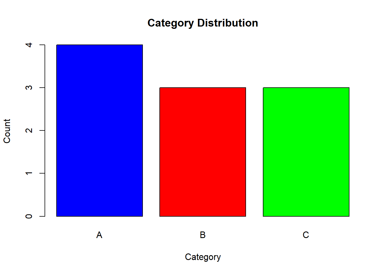
4.9.7 Exercise 7: Scatterplot with Regression Line
- Create two variables:
experience <- c(1, 2, 3, 4, 5, 6, 7, 8, 9, 10)
salary <- c(40000, 42000, 45000, 47000, 50000, 52000, 55000, 58000, 60000, 63000)- Create a scatterplot with a regression line.
Solution
plot(experience, salary, col = "blue", pch = 19, main = "Experience vs Salary",
xlab = "Years of Experience", ylab = "Salary ($)")
abline(lm(salary ~ experience), col = "red", lwd = 2)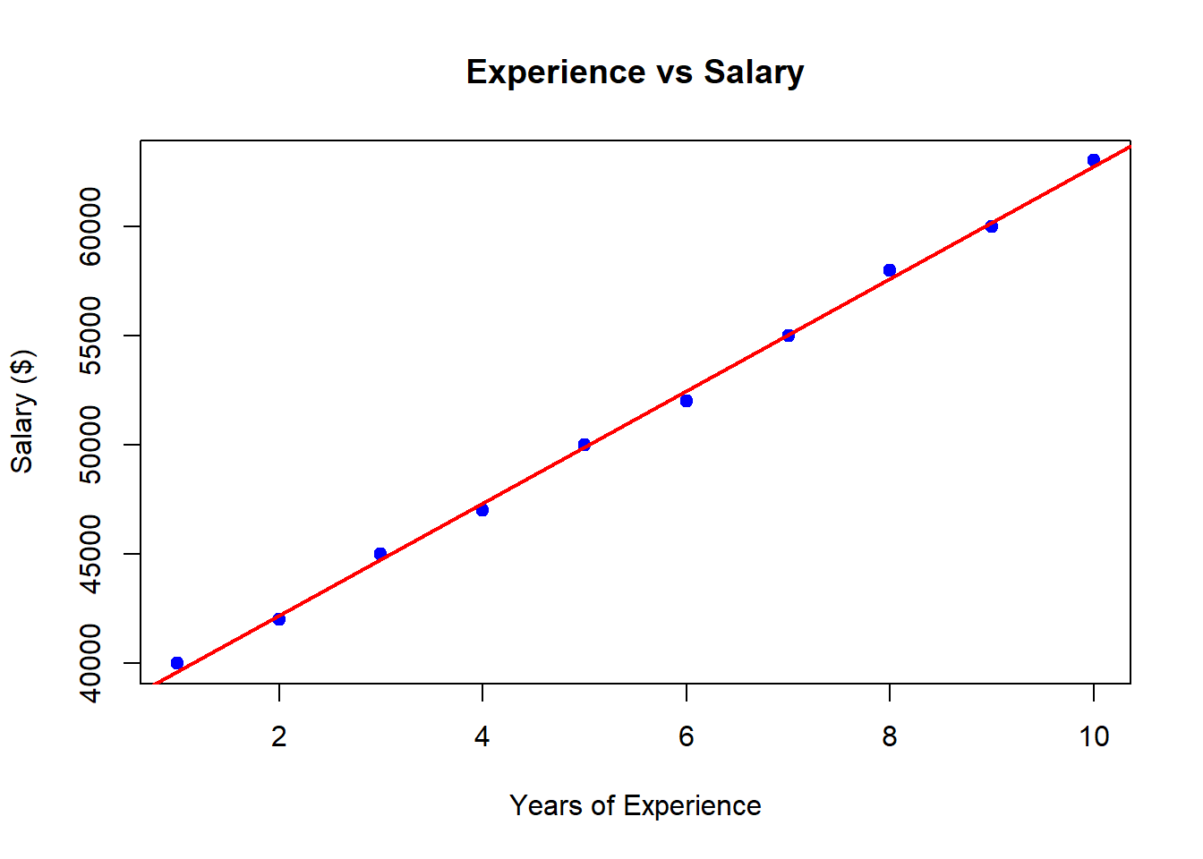
4.9.8 Exercise 8: Pairwise Comparisons
- Create a dataset with three groups:
group <- rep(c("Group A", "Group B", "Group C"), each = 5)
values <- c(85, 88, 90, 92, 94, 78, 80, 83, 85, 87, 70, 72, 75, 77, 79)- Perform pairwise t-tests.
Solution
##
## Pairwise comparisons using t tests with pooled SD
##
## data: values and group
##
## Group A Group B
## Group B 0.0085 -
## Group C 6.8e-05 0.0085
##
## P value adjustment method: holm4.9.9 Exercise 9: Tukey’s HSD Test
- Use the dataset:
treatment <- rep(c("Control", "Treatment A", "Treatment B"), each = 5)
response <- c(50, 55, 53, 52, 54, 60, 62, 65, 67, 64, 70, 72, 75, 78, 77)- Perform ANOVA and Tukey’s HSD test.
Solution
## Tukey multiple comparisons of means
## 95% family-wise confidence level
##
## Fit: aov(formula = response ~ treatment)
##
## $treatment
## diff lwr upr p adj
## Treatment A-Control 10.8 6.199708 15.40029 0.0001144
## Treatment B-Control 21.6 16.999708 26.20029 0.0000001
## Treatment B-Treatment A 10.8 6.199708 15.40029 0.00011444.9.10 Exercise 10: Comparing a Treatment to a Control
- A clinical trial tests three conditions:
condition <- rep(c("Control", "Low Dose", "High Dose"), each = 6)
blood_pressure <- c(130, 128, 132, 129, 131, 130, 125, 123, 120, 124, 126, 122, 115, 113, 118, 116, 117, 114)- Perform Dunnett’s test to compare treatments against the control.
Solution
# Ensure condition is a factor
condition <- factor(condition)
anova_model <- aov(blood_pressure ~ condition)
library(multcomp)
summary(glht(anova_model, linfct = mcp(condition = "Dunnett")))
##
## Simultaneous Tests for General Linear Hypotheses
##
## Multiple Comparisons of Means: Dunnett Contrasts
##
##
## Fit: aov(formula = blood_pressure ~ condition)
##
## Linear Hypotheses:
## Estimate Std. Error t value Pr(>|t|)
## High Dose - Control == 0 -14.500 1.063 -13.643 1.44e-09 ***
## Low Dose - Control == 0 -6.667 1.063 -6.273 2.90e-05 ***
## ---
## Signif. codes: 0 '***' 0.001 '**' 0.01 '*' 0.05 '.' 0.1 ' ' 1
## (Adjusted p values reported -- single-step method)________________________________________________________________________________