Chapter 5 LINEAR REGRESSION ANALYSIS
Regression is the finding of a relation between the input(predictor/independent) variable/s and the continuous output(target/dependent) variable.
Now Linear Regression is finding the linear relationship between dependent variable and one or more independent features by fitting a linear equation to the observed data. If there is one independent variable therefore the regression in known as simple linear regression while if multiple variables are involved it is known as multiple linear regression.
5.1 Simple Linear Regression Analysis
Simple linear regression seeks to explore and model the relationship between two quantitative variables. Here’s what it helps you do:
- Understand the strength of the relationship:
For example, it can reveal how strongly rainfall affects soil erosion. If the relationship is strong, changes in rainfall levels are likely to lead to significant changes in soil erosion.
- Make predictions:
It allows you to estimate the dependent variable’s value for a given value of the independent variable. For instance, if you know how much it rained, you can predict how much soil erosion occurred.
The beauty of simple linear regression lies in its simplicity—you’re working with just two variables. One acts as the input, and the other as the output. It’s like finding a straight-line path that best connects the data points and helps explain their relationship.
For instance, imagine plotting rainfall (in mm) on the x-axis and soil erosion (in kg) on the y-axis. A regression line (a straight line) is fitted to the data, showing the trend. If the line slopes upwards, it means more rain leads to more soil erosion—a positive relationship. If it slopes downward, it’s a negative relationship.
So, simple linear regression isn’t just math—it’s a way to uncover insights and make informed predictions from real-world data!
5.1.1 Empirical model-building-regression analysis
Simple linear regression is a parametric test, which means it relies on certain assumptions about your data to ensure accurate and reliable results. Let’s break down these assumptions:
Key Assumptions of Simple Linear Regression
- Homogeneity of variance (Homoscedasticity):
The prediction errors (residuals) should remain roughly the same across all values of the independent variable. In simpler terms, the “spread” of data points around the regression line should stay consistent, not get wider or narrower.
- Independence of observations:
Each data point in your dataset should be collected independently. For example, there shouldn’t be hidden relationships or patterns among your observations, like duplicate measurements or a biased sampling method.
- Normality:
The data (especially the residuals) should follow a normal distribution. This is important for making valid inferences from your model.
- Linearity:
The relationship between the independent and dependent variables should be linear. That means the best-fitting line through your data points should be straight, not curved or clustered into groups.
What if these assumptions aren’t met?
If your data violate assumptions like homoscedasticity or normality, don’t worry—you still have options! For instance, you can use a nonparametric test like the Spearman rank test, which doesn’t rely on strict parametric assumptions.
By ensuring your data meets these conditions, you can confidently use simple linear regression to model and predict relationships between variables!
The formula for simple linear regression looks like this: \[y = \alpha + \beta X + \epsilon\]
where;
- \(y\): the predicted value of the dependent variable.
- \(X\): the independent variable believed to be influencing the value of \(y\)
- \(\alpha\): the intercept, or the starting point. It tells you the predicted value of \(y\) when \(X\) (the independent variable) is 0.
- \(\beta\): the regression coeefficient, which measures the expected change in \(y\) for each one unit increase in \(X\). This is the slope/gradient of the line.
- \(\epsilon\): the error term, representing how much actual data points deviate from the predicted line.
This is how linear regression works:
Linear regression fits a line of best fit through your data points. It finds the value of \(\beta\) (the slope) that minimizes the total error (the difference between the observed and predicted values of \(y\).
In simple terms, the regression line represents the most accurate straight-line relationship between your independent variable (\(X\)) and your dependent variable (\(y\)).
Try it!
Lets make this practical, you will be required to download the plant height data from here.
Remember: The goal in linear regression is obtain the best estimates for the model coefficients(\(\alpha\) and \(\beta\)).
We will break down the process in steps;
- Load the data set
The goal of this analysis is to find the linear association between the plant height and the temperature, particularly if plant height is dependent on the temperature.
Define the independent and dependent variables: temperature(
temp) is the independent variable while plant height(loght) is the dependent variable
##
## Call:
## lm(formula = loght ~ temp, data = df)
##
## Coefficients:
## (Intercept)         temp
##    -0.22566      0.04241
5.1.2 Interpreting the regression results
To get a detailed breakdown of the regression results, such as the coefficient values, \(R^2\), test statistics, p-values, and confidence intervals, you need to save the output of the lm function to an object. Then, use the summary() function on that object to extract and review the analysis details.
Note: loght is log(plant height).
##
## Call:
## lm(formula = loght ~ temp, data = df)
##
## Residuals:
##      Min       1Q   Median       3Q      Max
## -1.97903 -0.42804 -0.00918  0.43200  1.79893
##
## Coefficients:
##              Estimate Std. Error t value Pr(>|t|)
## (Intercept) -0.225665   0.103776  -2.175    0.031 *
## temp         0.042414   0.005593   7.583 1.87e-12 ***
## ---
## Signif. codes:  0 '***' 0.001 '**' 0.01 '*' 0.05 '.' 0.1 ' ' 1
##
## Residual standard error: 0.6848 on 176 degrees of freedom
## Multiple R-squared:  0.2463, Adjusted R-squared:  0.242
## F-statistic:  57.5 on 1 and 176 DF,  p-value: 1.868e-12
The regression output provides the slope and intercept of the regression line. Based on this analysis, the regression equation for predicting the (log-transformed) plant height as a function of temperature is:
\[loght = −0.22566+0.04241*temp + \epsilon\]
and this is the breakdown of the analysis;
- Coefficients
The intercept (-0.22566) represents the predicted value of log(plant height) when the temperature is zero.
The slope (0.04241) indicates that for every one-unit increase in temperature, the log(plant height) increases by approximately 0.04241.
- Significance of Coefficients
The t-statistics and p-values test whether the coefficients are significantly different from zero.
Here, the p-value for temperature (< 0.005) suggests a statistically significant relationship between temperature and plant height.
The intercept’s p-value (0.031) is less important since we typically focus on the slope’s significance.
- Overall Model Significance
The F-statistic (57.5) and its associated p-value (<0.001) confirm that the overall model is statistically significant.
With a single predictor, the p-value for the F-statistic is identical to the p-value for the slope coefficient.
5.1.3 R-squared and Adjusted R-Squared
R-squared, or the coefficient of determination, measures the proportion of the variance in the dependent variable (\(y\)) that is explained by the independent variable(s) (\(x\)) in a regression model. It is a goodness-of-fit statistic.
On the other hand, Adjusted R-squared modifies R-squared to account for the number of predictors in the model, providing a more accurate measure of model performance, especially for multiple regression.
Like our model above shows that:
- The \(R^2\) value (0.2463) shows that approximately 24.6% of the variation in plant height is explained by temperature.
- The adjusted \(R^2\) (0.242) slightly adjusts for the model’s complexity and is more relevant when comparing models
Practical Exercise
You will be provided the creek_basin_data.csv file by your instructor. The data is about the effect of the amount of rainfall on the creek run off. The objective is to investigate for a linear relationship between the amount of rainfall and the creek run off. You are required to;
- Build a simple linear regression model
- Evaluate R-squared and Adjusted r-squared to find if the the linear model is effective.
- Finally, visualize the model
Solution
- Build a simple linear regression model
# Load the data
creek_data <- read.csv("data/creek_basin_data.csv")

# Fit linear regression model
model <- lm(Runoff_cm ~ Rainfall_cm, data = creek_data)

# Display model summary
summary(model)
##
## Call:
## lm(formula = Runoff_cm ~ Rainfall_cm, data = creek_data)
##
## Residuals:
## Min 1Q Median 3Q Max
## -4.4759 -1.2265 -0.0395 1.1927 4.4345
##
## Coefficients:
## Estimate Std. Error t value Pr(>|t|)
## (Intercept) 0.01801 0.51541 0.035 0.972
## Rainfall_cm 0.69281 0.02735 25.335 <2e-16 ***
## ---
## Signif. codes: 0 '***' 0.001 '**' 0.01 '*' 0.05 '.' 0.1 ' ' 1
##
## Residual standard error: 1.939 on 98 degrees of freedom
## Multiple R-squared: 0.8675, Adjusted R-squared: 0.8662
## F-statistic: 641.9 on 1 and 98 DF, p-value: < 2.2e-16The regression line equation inform of \(y = \alpha + \beta x + \epsilon\) goes by; \[\text Runoff = 0.01801 + 0.69281 \times Rainfall + \epsilon\] This means that a 0cm rain would yield to approximately 0.01801cm runoff The p-value for rainfall is \(2 \times 10^{-16}\), meaning that the rainfall is a significant predictor for ruin off
- Evaluate R-squared and Adjusted r-squared to find if the the linear model is effective.
# Extract R-squared and Adjusted R-squared to present it clearly
r_squared <- summary(model)$r.squared
adjusted_r_squared <- summary(model)$adj.r.squared

cat("R-Squared:", r_squared, "\n")
## R-Squared: 0.8675463## Adjusted R-Squared: 0.8661947The Multiple r-squared = 08675, that is approximately 87% of the variability in runoff is explained by rainfall. Since it is a simple linear regression problem and we only have one predictor, R² and Adjusted R² are very close.
- Finally, visualize the model
# Load the required library
library(ggplot2)

# Scatter plot with regression line
ggplot(creek_data, aes(x = Rainfall_cm, y = Runoff_cm)) +
  geom_point() +
  geom_smooth(method = "lm", col = "blue") +
  labs(title = "Rainfall vs Runoff", x = "Rainfall (cm)", y = "Runoff (cm)")
## `geom_smooth()` using formula = 'y ~ x'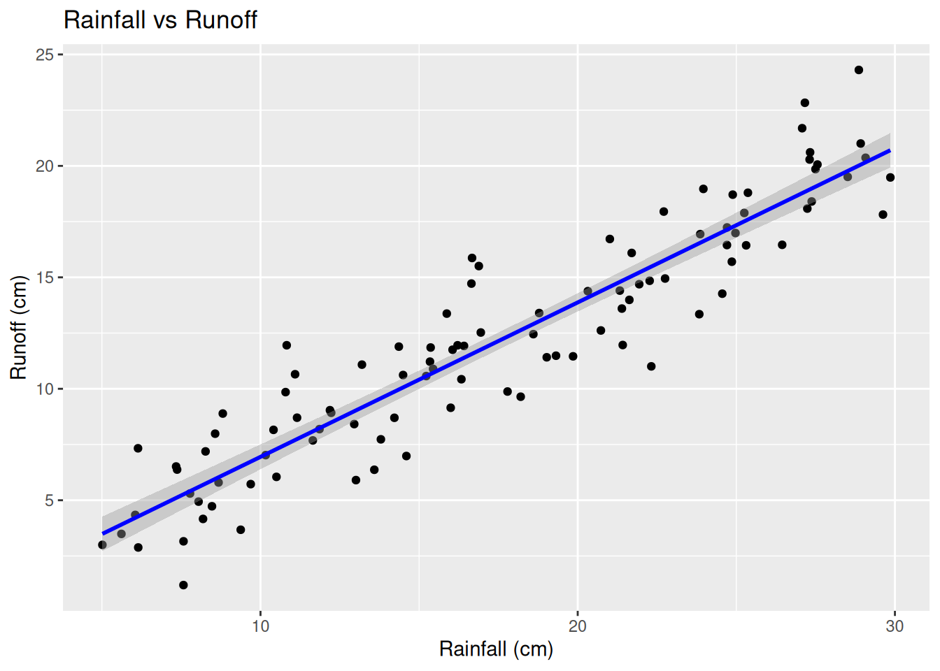
________________________________________________________________________________
5.2 Data transformation versus generalized linear model
5.2.1 Data Transformation Approach (Log Transformation)
In this sub-course, we will consider a study where we examine how pollution levels affect fish abundance in a river system. We assume:
- Low pollution results in higher fish abundance.
- High pollution results in lower fish abundance.
- Fish abundance is a count variable (discrete, non-negative).
Ecological data is often skewed (many low values, few high values). Log transformation stabilizes variance and makes the distribution closer to normal: \[Y'= log(Y + 1)\] where;
- \(Y'\) is the transformed fish abundance
- \(Y\) is the original fish abundance (adding 1 prevents log(0)).
A linear regression model can be used after transformation: \[log(Y+1) = \beta_0 + \beta_1X + \epsilon\] as described. However transformation posses with several limitations such as;
- Interpretation is difficult because the response variable is no longer on the original scale.
- Transformation may not fully address skewness in highly non-normal data.
- Not ideal for count data, which follow discrete probability distributions.
5.2.2 Generalized Linear Model(GLM)
Instead of transforming the data, we can use a Poisson regression model, which assumes that fish abundance follows a Poisson distribution: \[Y \text ~ Poisson(\lambda)\] where \(Y\) is the data value count(count of observed fish) and \(\lambda\) is the expected abundance(fish abundance in our case)
GLMs use a log-link function to model the expected count directly: \[log(\lambda) = \beta_0 + \beta_1X\] Solving for \(\lambda\); \[\lambda = e^{\beta_o + \beta_1X}\] Keep in mind that;
- \(e^{\beta_o}\) is the expected abundance in low pollution areas
- \(e^{\beta_1X}\) is the multiplicative effect of pollution.
GLM(Poisson Regression model) posses various advantages where it;
- Maintains original scale of the response variable (counts).
- is more appropriate for count data, which are often non-normal.
- Exponential interpretation: \(e^{\beta_1}\) gives the factor by which abundance changes due to pollution.
Try it!
Lets simulate the fish population in respect to pollution levels using R.
Step 1: Generate the data
# Load necessary libraries
library(ggplot2)
library(dplyr)

# Set seed for reproducibility
set.seed(123)

# Simulate pollution levels (Low = 0, High = 1)
n <- 100  # Number of observations
pollution <- sample(0:1, n, replace = TRUE)

# Generate fish abundance (count data)
fish_abundance <- rpois(n, lambda = ifelse(pollution == 0, 15, 5)) # Lower in polluted areas

# Combine into a data frame
data <- data.frame(Pollution = factor(pollution, levels = c(0, 1), labels = c("Low", "High")),
                   Fish_Abundance = fish_abundance)

# Check its distribution
hist(data$Fish_Abundance)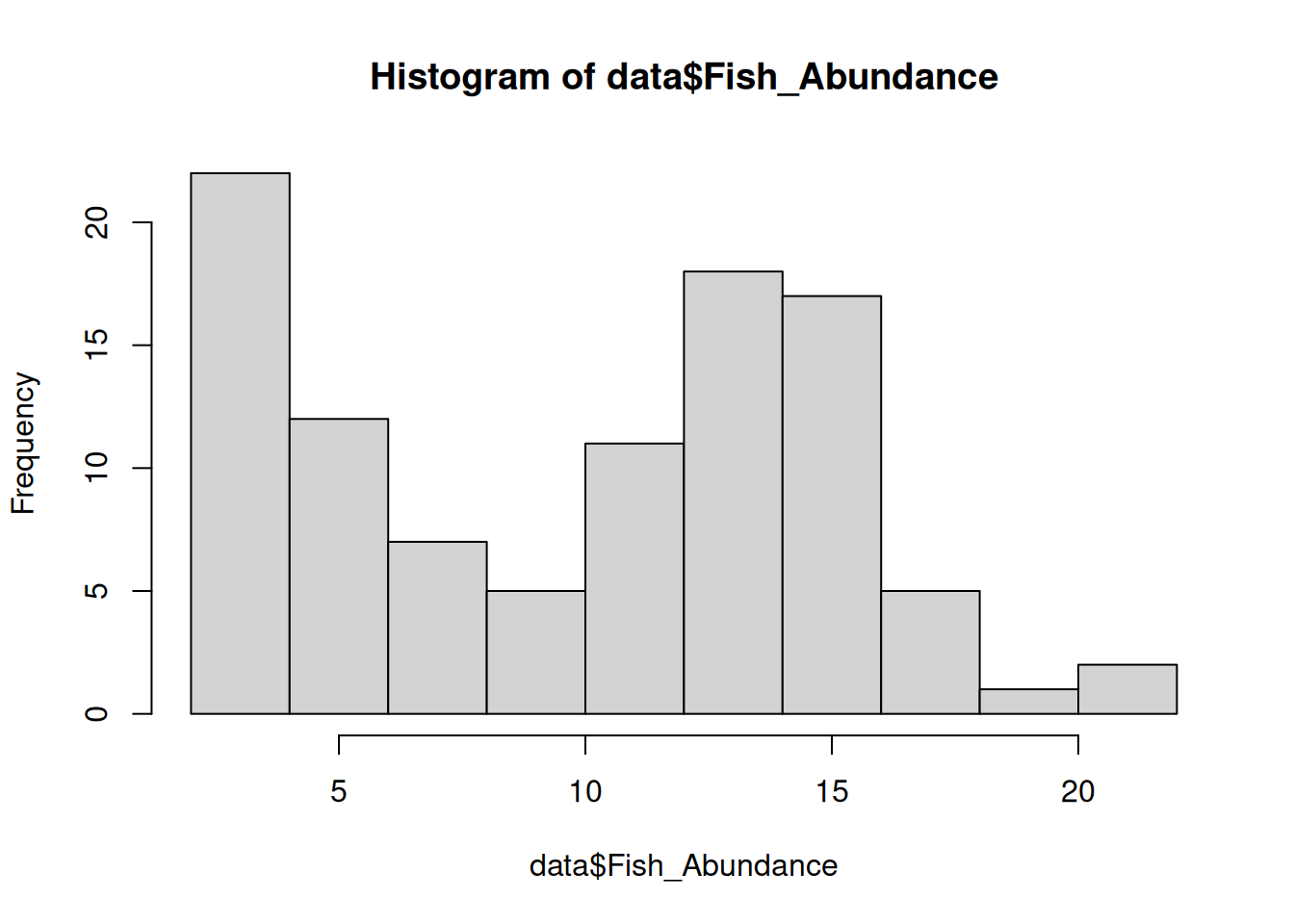
##  Pollution Fish_Abundance
##  Low :57   Min.   : 2.00
##  High:43   1st Qu.: 5.00
##            Median :11.50
##            Mean   :10.26
##            3rd Qu.:14.25
##            Max.   :22.00
Apply log transformation since the data is right-skewed
# Log transform fish abundance (add 1 to avoid log(0))
data$Log_Abundance <- log(data$Fish_Abundance + 1)

# Boxplot to visualize transformed vs. untransformed data
ggplot(data, aes(x = Pollution, y = Fish_Abundance)) +
  geom_boxplot() +
  labs(title = "Raw Fish Abundance vs. Pollution Level") +
  theme_minimal()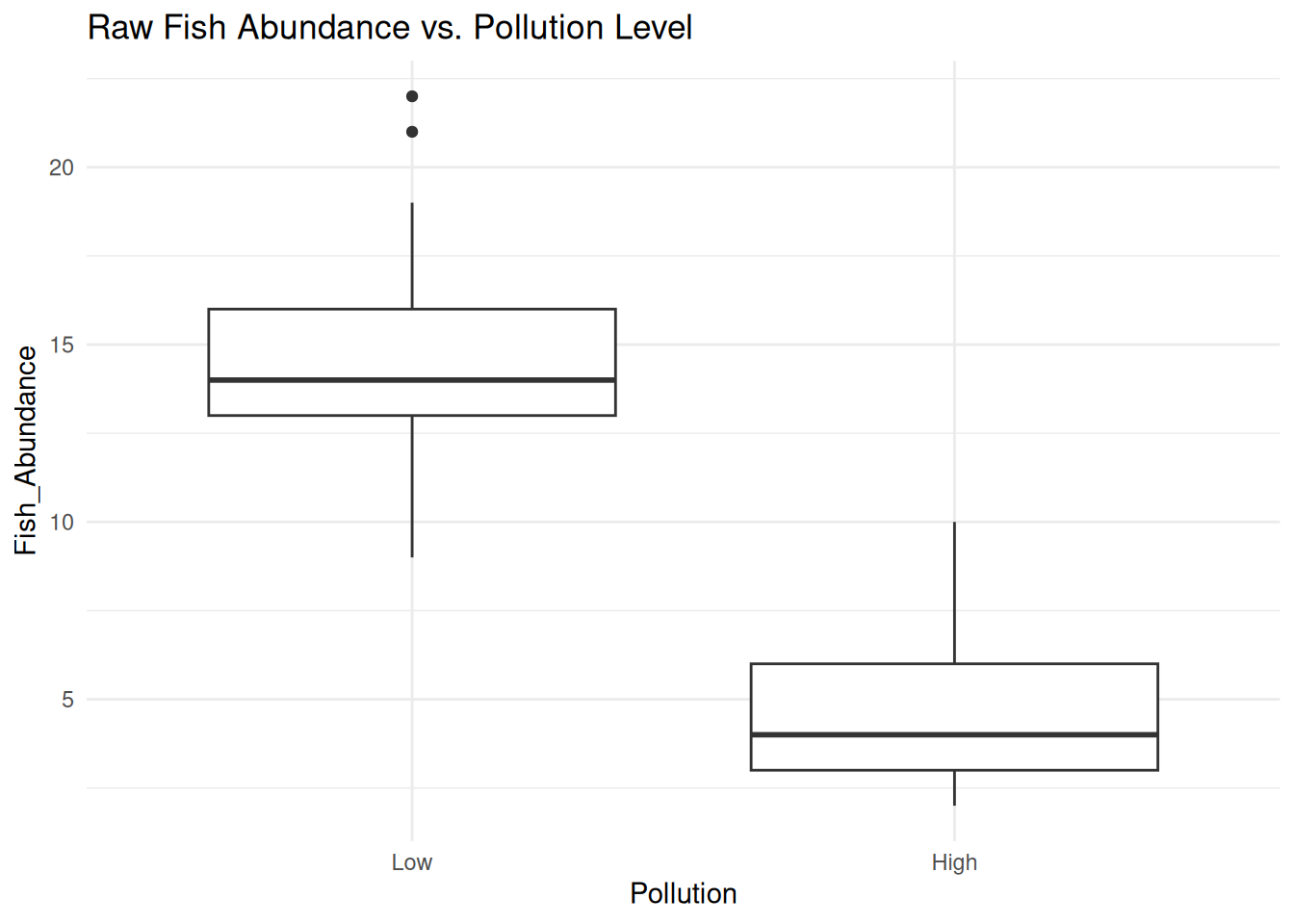
ggplot(data, aes(x = Pollution, y = Log_Abundance)) +
geom_boxplot(fill = "lightblue") +
labs(title = "Log-Transformed Fish Abundance vs. Pollution Level") +
theme_minimal()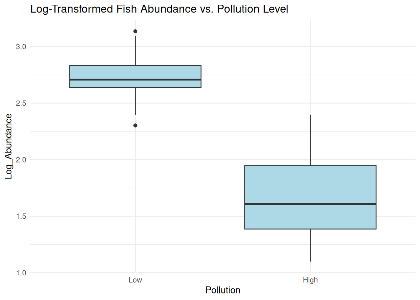 The log transformation helps stabilize variance and make the distribution more normal.
However, using transformed data in regression may not always be statistically appropriate for count data.
The log transformation helps stabilize variance and make the distribution more normal.
However, using transformed data in regression may not always be statistically appropriate for count data.
Instead of transforming, we use a Poisson (GLM), which is designed for count data.
# Fit Poisson GLM
glm_model <- glm(Fish_Abundance ~ Pollution, family = poisson, data = data)

# Model summary
summary(glm_model)
##
## Call:
## glm(formula = Fish_Abundance ~ Pollution, family = poisson, data = data)
##
## Coefficients:
## Estimate Std. Error z value Pr(>|z|)
## (Intercept) 2.66014 0.03503 75.94 <2e-16 ***
## PollutionHigh -1.06948 0.07724 -13.85 <2e-16 ***
## ---
## Signif. codes: 0 '***' 0.001 '**' 0.01 '*' 0.05 '.' 0.1 ' ' 1
##
## (Dispersion parameter for poisson family taken to be 1)
##
## Null deviance: 289.134 on 99 degrees of freedom
## Residual deviance: 59.428 on 98 degrees of freedom
## AIC: 465.3
##
## Number of Fisher Scoring iterations: 4The Poisson model directly models count data without transformation. The coefficient for “High Pollution” = -1.06948 shows how pollution reduces fish abundance in a statistically valid way. A negative correlation where increase in pollution results in decrease in fish abundance and vice versa.
Practical Exercise
Using the creek_basin_data.csv, Log transform the data and fit with a generalized linear model. If the the transformation improves the R-squared value(from the simple linear regression model), then its is more appropriate(Shows the residuals may not be normally distributed)
Solution
Lets log transform the data
# Apply log transformation to both variables
creek_data$log_Rainfall <- log(creek_data$Rainfall_cm)
creek_data$log_Runoff <- log(creek_data$Runoff_cm)

# Fit linear model with log-transformed data
log_model <- lm(log_Runoff ~ log_Rainfall, data = creek_data)
summary(log_model)
##
## Call:
## lm(formula = log_Runoff ~ log_Rainfall, data = creek_data)
##
## Residuals:
## Min 1Q Median 3Q Max
## -1.42140 -0.09909 0.01952 0.10424 0.61348
##
## Coefficients:
## Estimate Std. Error t value Pr(>|t|)
## (Intercept) -0.52368 0.14773 -3.545 0.000604 ***
## log_Rainfall 1.04825 0.05274 19.877 < 2e-16 ***
## ---
## Signif. codes: 0 '***' 0.001 '**' 0.01 '*' 0.05 '.' 0.1 ' ' 1
##
## Residual standard error: 0.2447 on 98 degrees of freedom
## Multiple R-squared: 0.8013, Adjusted R-squared: 0.7992
## F-statistic: 395.1 on 1 and 98 DF, p-value: < 2.2e-16The model above captures the nonlinear relationship of the rainfall amount the run off, however it is a lower accuracy than the simple linear model. Accuracy reduced by 0.05 which is 5%.
Now we fit a generalized Linear model
# Fit GLM (Gaussian with identity link function)
glm_model <- glm(Runoff_cm ~ Rainfall_cm, family = gaussian(link = "identity"), data = creek_data)
summary(glm_model)
##
## Call:
## glm(formula = Runoff_cm ~ Rainfall_cm, family = gaussian(link = "identity"),
## data = creek_data)
##
## Coefficients:
## Estimate Std. Error t value Pr(>|t|)
## (Intercept) 0.01801 0.51541 0.035 0.972
## Rainfall_cm 0.69281 0.02735 25.335 <2e-16 ***
## ---
## Signif. codes: 0 '***' 0.001 '**' 0.01 '*' 0.05 '.' 0.1 ' ' 1
##
## (Dispersion parameter for gaussian family taken to be 3.758101)
##
## Null deviance: 2780.55 on 99 degrees of freedom
## Residual deviance: 368.29 on 98 degrees of freedom
## AIC: 420.16
##
## Number of Fisher Scoring iterations: 2The GLM results are almost identical to the original linear model and the AIC = 420.16 confirms a relatively good model fit, though the log-transformed model had a stronger R².
If the residuals in the original linear model are not normal, the GLM can handle that better.
________________________________________________________________________________
5.3 Multiple Linear Regression (MLR) model
Unlike simple linear regression, multiple linear regression describes the linear relationship between two or more independent variables with one target(dependent) variable. The objective of multiple linear regression is to;-
- Find the strength of the relationship between two or more independent variables with the target variables.
- Find the value of the target variable at a certain value of the independent variable.
When working on a multiple linear regression it is assumed that; the variance is homogeneous such that the prediction error does not change significantly across the predictor(independent) variables. It is also assumed, observations were independent and there was no hidden relationships among the variables when collecting the data. Additionally, the collected data follows a normal distribution and the independent variables have a linear relationship(linearity) with the dependent variable, therefore, the line of best fit through the data points is straight and not curved.
Multiple linear regression is modeled by;-

where;-
- \(y\) is the predicted value of the target variable.
- \(\beta_0\) is the y-intercept. Value of y when all other parameters are zero.
- \(\beta_1X_1\): \(\beta_1\) is the regression coefficient of the first independent variable while \(X_1\) is the independent variable value. \(\cdots\) do the same for however the number of independent variables are present.
- \(\beta_nX_n\): the regression coefficient of the last independent variable.
- \(\epsilon\) is the model error(variation not explained by the independent variables)
The Multiple linear regression model calculates three things to find the best fit line for each independent variable;-
- The regression coefficient \(\beta_iX_i\) that will minimize the overall error rate(model error).
- The associated p-value. If the relationship between the independent variable is statistically significant.
- The t-statistic of the model. T-statistic is the ratio of the difference in a number’s estimated value from its assumed value to its standard error.
——add an example ——————————
——Add Assumptions of Multiple Linear Regression———————-
Practical exercise
Using the airquality data set, fit a multiple linear regression model whereby the Solar radiation(Solar.R), Ozone and Wind are the independent variables while the Temperature (Temp) is the dependent variable. Interpret and analyze the results
5.4 Hands-on Exercise
In this exercise, we will utilize the Global Species Abundance and Diversity data set that can be downloaded from here. It comprises of different species and diversity from different ecological sites, offering a global perspective on biodiversity
——————————————————————-Will be revisited ——————————————————–
Solution
________________________________________________________________________________