6 Steps in Species Distribution Modeling (SDM)
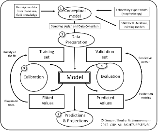
In this section, we break down the five critical steps in building a Species Distribution Model (SDM). Each step has unique goals, methodologies, and challenges that guide you through understanding and predicting species distributions.
— ***** ## Step 1: Conceptualization Objective: Define the research question and identify both biological and environmental data needs.
6.0.1 Key Points to Consider
6.0.1.1 1. Research Design
A well-thought-out research design ensures your SDM focuses on the species and factors that matter most. Ask yourself:
-
What species are you studying?
- Are you focusing on a rare or endangered species?
- Does the species have ecological or economic importance?
- Are there known relationships between the species and specific environmental variables?
- Are you focusing on a rare or endangered species?
-
Which environmental factors (predictors) are likely to influence its distribution?
- Consider variables that directly or indirectly affect the species:
-
Direct factors: Temperature, precipitation, soil type.
-
Indirect factors: Elevation, aspect, vegetation cover.
-
Direct factors: Temperature, precipitation, soil type.
- Identify predictors based on ecological theory or prior studies.
- Consider variables that directly or indirectly affect the species:
6.0.1.2 2. Data Sources
To ensure data quality and relevance, rely on a combination of biological and environmental data sources:
-
Biological Data Sources:
-
Field Observations:
- Use surveys, citizen science data (e.g., iNaturalist, eBird), or camera trap records.
- Ensure data is georeferenced with accurate longitude and latitude.
-
Historical Records:
- Extract data from herbarium specimens, museum records, or published literature.
-
Field Observations:
-
Environmental Data Sources:
-
Remote Sensing Datasets:
- Gather variables like land cover, vegetation indices (e.g., NDVI), and soil moisture from satellites like MODIS or Landsat.
-
Global Climate Datasets:
- Use datasets like WorldClim, CHELSA, or CMIP6 to extract temperature, precipitation, or bioclimatic variables.
-
Remote Sensing Datasets:
Example Sources:
- Biological data: GBIF for occurrence records.
- Environmental data: WorldClim for climate variables (e.g., annual mean temperature, precipitation).
6.0.1.3 3. Assumptions
Every SDM is built on ecological and statistical assumptions. Identifying and addressing these assumptions ensures model reliability:
-
Ecological Assumptions:
- The species is in equilibrium with its environment (i.e., the distribution reflects its ecological preferences).
- The environmental variables included in the model are sufficient to explain its distribution.
- The species is in equilibrium with its environment (i.e., the distribution reflects its ecological preferences).
-
Data Assumptions:
- Absence data (if available) reflects true absences rather than sampling gaps.
- Presence-only data (p-o) is not overly biased by sampling effort or geographic bias.
- Absence data (if available) reflects true absences rather than sampling gaps.
-
Modeling Assumptions:
- The chosen algorithm can capture the species-environment relationships effectively.
- Predictors are independent of each other (e.g., no collinearity).
- The chosen algorithm can capture the species-environment relationships effectively.
6.0.2 Practical Example: Eastern Hemlock (Tsuga canadensis)
Let’s conceptualize an SDM for eastern hemlock, a late-successional conifer in North America.
-
Research Design:
- Question: How will climate change affect the future distribution of Tsuga canadensis?
- Predictors: Key variables might include:
-
Climate: Annual mean temperature (Bio1), precipitation seasonality (Bio15).
-
Topography: Elevation, slope, aspect.
- Soil Characteristics: Drainage class, organic content.
-
Climate: Annual mean temperature (Bio1), precipitation seasonality (Bio15).
- Question: How will climate change affect the future distribution of Tsuga canadensis?
-
Data Sources:
- Biological data: Combine presence-absence data from field surveys with occurrence records from GBIF.
- Environmental data: Use WorldClim bioclimatic variables and a digital elevation model (DEM).
- Biological data: Combine presence-absence data from field surveys with occurrence records from GBIF.
-
Assumptions:
- The distribution of Tsuga canadensis is primarily limited by climate and soil factors.
- Presence records accurately represent locations where the species occurs under current climate conditions.
- The distribution of Tsuga canadensis is primarily limited by climate and soil factors.
6.0.3 Why Conceptualization Matters
Proper conceptualization ensures the SDM focuses on biologically meaningful relationships and avoids common pitfalls like using irrelevant predictors or biased occurrence data. It lays the groundwork for robust, interpretable models that can inform conservation and management strategies.
Pro Tip: Use a literature review to identify relevant predictors and validate your assumptions. This saves time and ensures your model is grounded in existing ecological knowledge.
6.1 Step 2: Data Preparation
Objective: Gather, clean, and process both biological and environmental data to ensure they are ready for modeling.
6.2 Data preparation is a critical step in Species Distribution Modeling (SDM). The quality of your input data significantly influences the accuracy and reliability of the resulting model. This step involves cleaning and processing both biological (species occurrence) data and environmental predictors.
6.2.1 Key Tasks
6.2.1.1 1. Preparing Biological Data
Biological data forms the basis for understanding species distributions. It can come in two main formats:
-
Presence-Only (p-o): Records of where the species has been observed but with no information on absence (e.g., citizen science data from GBIF).
- Presence-Absence (p-a): Data explicitly indicating locations where the species is present or absent (e.g., survey data).
Steps for Cleaning Biological Data: - Remove Duplicates: - Ensure there are no duplicate records, especially for presence data.
- Duplicates can over-represent certain locations and bias the model. - Fix Erroneous Coordinates: - Check for invalid or missing latitude/longitude values. - Remove records with extreme outliers (e.g., points plotted in the ocean for terrestrial species). - Address Spatial Bias: - Sampling effort can vary across regions. Use techniques like spatial thinning to reduce over-representation of areas with high sampling intensity.
Tool Spotlight: Use packages like CoordinateCleaner in R to identify and clean problematic occurrence records, such as duplicates or points in impossible locations.
6.2.1.2 2. Preparing Environmental Data
Environmental data consists of predictors that describe the abiotic and biotic conditions influencing species distributions. These predictors are typically derived from:
-
Climate Variables: Temperature, precipitation, seasonality (e.g., from WorldClim or CMIP6).
-
Topographic Variables: Elevation, slope, aspect (e.g., from DEMs).
- Land Cover: Vegetation type, NDVI (e.g., from MODIS or ESA datasets).
Key Considerations: - Alignment: - Ensure that all raster layers (predictors) have the same: - Resolution: Each raster cell should represent the same area (e.g., 10 km × 10 km).
- Extent: All rasters should cover the same geographic boundaries.
- CRS: Use the same coordinate reference system (e.g., WGS84).
- Quality Check: - Inspect rasters for missing or unrealistic values (e.g., negative precipitation).
Why Alignment Matters: Mismatched resolution, extent, or CRS can lead to errors during spatial analysis, such as misaligned layers or invalid predictions.
6.2.1.3 3. Scaling and Temporal Matching
Temporal and spatial consistency between biological and environmental data is essential for robust modeling:
-
Temporal Alignment:
- Biological data (e.g., species occurrences) and environmental data (e.g., climate variables) should reflect the same time period.
- Example: If occurrence data is from 2020, use climate data from the same year or a comparable period.
- Biological data (e.g., species occurrences) and environmental data (e.g., climate variables) should reflect the same time period.
-
Scaling:
- Standardize numerical predictors (e.g., z-scores or min-max scaling) to ensure all variables contribute equally to the model.
Watch Out For: - Predictors with different temporal scales (e.g., historical vs. future climate data).
- Variables with units that aren’t comparable (e.g., temperature in °C vs. precipitation in mm).
6.2.2 Pro Tip: Checking Multicollinearity
Multicollinearity occurs when predictors are highly correlated, which can distort the model’s ability to attribute importance to variables. Common examples include: - Annual mean temperature (Bio1) and maximum temperature of the warmest month (Bio5). - Annual precipitation (Bio12) and precipitation seasonality (Bio15).
How to Address It: - Calculate a correlation matrix for your predictors and remove one variable from each highly correlated pair (e.g., correlation > 0.7). - Use dimensionality reduction techniques like Principal Component Analysis (PCA) to summarize predictors into uncorrelated components.
Tool Spotlight: Use the vif() function from the car package to identify predictors with high variance inflation factors (VIF), which indicate multicollinearity.
6.2.3 Example: Preparing Data for Eastern Hemlock SDM
To model the distribution of eastern hemlock (Tsuga canadensis), you would:
-
Biological Data:
- Download occurrence records from GBIF.
- Remove duplicates and points with missing or invalid coordinates.
- Thin the data spatially to reduce sampling bias.
- Download occurrence records from GBIF.
-
Environmental Data:
- Download bioclimatic variables (e.g., Bio1: Annual Mean Temperature, Bio12: Annual Precipitation) from WorldClim.
- Align rasters to a common resolution of 10 km × 10 km, with the WGS84 CRS.
- Download bioclimatic variables (e.g., Bio1: Annual Mean Temperature, Bio12: Annual Precipitation) from WorldClim.
-
Scaling and Matching:
- Standardize climate variables (e.g., z-scores).
- Ensure climate data corresponds to the same year as the occurrence data.
- Standardize climate variables (e.g., z-scores).
6.2.4 Why Data Preparation Matters
High-quality data is the backbone of any SDM. Poorly prepared data can lead to: - Biased or inaccurate predictions. - Overfitting, where the model learns noise rather than meaningful patterns. - Misleading conservation decisions based on faulty models.
Checklist for Data Preparation: 1. Biological Data: - Remove duplicates and erroneous coordinates. - Address spatial bias in occurrence data. 2. Environmental Data: - Align predictors (resolution, extent, CRS). - Standardize numerical variables. 3. Temporal Matching: - Ensure biological and environmental data reflect the same time period. 4. Multicollinearity Check: - Remove or reduce highly correlated predictors.
6.3 Step 3: Model Fitting
Objective: Select and apply the most appropriate modeling algorithm to fit the SDM, ensuring the model captures meaningful species-environment relationships while avoiding overfitting.
6.4 Model fitting is the core step in SDM, where the relationship between species occurrence and environmental predictors is quantified. The choice of algorithm and careful selection of predictors are critical to building an accurate and interpretable model.
6.4.1 Key Considerations
6.4.1.1 1. Algorithm Selection
Different algorithms are suitable for different data types and modeling goals. Choose an algorithm based on your biological data type (e.g., presence-only or presence-absence) and the complexity of the study.
| Algorithm | Data Type | Strengths | Example Use Case |
|---|---|---|---|
| MaxEnt | Presence-Only (p-o) | Handles small sample sizes and generates robust results. | Predicting distributions using citizen science data. |
| Random Forest (RF) | Presence-Absence (p-a) | Handles nonlinear relationships and interactions. | Modeling habitat suitability with complex predictors. |
| GLMs/GAMs | Presence-Absence (p-a) | Parametric models for interpretable relationships. | Studying simple, linear species-environment responses. |
| Boosted Regression Trees (BRT) | Presence-Absence (p-a) | Handles missing data and identifies important variables. | Predicting species presence in highly variable landscapes. |
Pro Tip: Start with a simple model (e.g., GLM) to establish baseline performance and then explore more complex algorithms like RF or BRT for improved accuracy.
6.4.1.2 2. Variable Selection
Careful selection of predictors ensures your model captures meaningful relationships without overfitting. Multicollinearity (high correlation between predictors) can distort the model’s interpretation and reliability.
Steps for Variable Selection: 1. Check for Multicollinearity: - Calculate a correlation matrix or Variance Inflation Factor (VIF) for predictors. - Remove one variable from each pair with correlation > 0.7 (e.g., Bio1 and Bio5 in climate data).
-
Prioritize Ecological Relevance:
- Retain variables that are biologically relevant to the species’ niche.
- Example: For eastern hemlock (Tsuga canadensis), focus on predictors like temperature seasonality (Bio4) and annual precipitation (Bio12).
-
Iterative Refinement:
- Test the model’s performance with different sets of predictors.
- Use techniques like backward elimination or stepwise selection to identify the best set.
Example: If you have 19 bioclimatic variables from WorldClim, select only a subset (e.g., 4–6 variables) based on their correlation and ecological significance.
6.4.1.3 3. Overfitting Avoidance
Overfitting occurs when the model becomes too complex and performs well on training data but poorly on unseen data. Avoid overfitting using the following strategies:
-
Regularization:
- In MaxEnt, adjust the regularization multiplier to penalize overly complex models.
-
Cross-Validation:
- Split the data into training and testing subsets (e.g., 70% training, 30% testing).
- Use k-fold cross-validation to evaluate the model on multiple splits of the data.
-
Simplify the Model:
- Avoid using too many predictors, especially if sample size is small.
- Example: For a dataset with 100 species occurrence records, limit the predictors to ~5–6 variables.
Watch Out For: - Using all available predictors without assessing collinearity. - Relying solely on training accuracy without testing the model on independent data.
6.4.2 Example: Fitting a Model for Eastern Hemlock
For the eastern hemlock (Tsuga canadensis), we aim to understand how environmental factors influence its distribution:
-
Data:
- Presence-absence records of the species across North America.
- Bioclimatic predictors (e.g., Bio4: Temperature Seasonality, Bio12: Annual Precipitation).
-
Algorithm:
- Use Random Forest (RF) due to its ability to handle complex, nonlinear relationships.
-
Variable Selection:
- Start with all 19 bioclimatic variables.
- Remove highly correlated variables (e.g., Bio1 and Bio5).
- Retain key predictors based on ecological knowledge.
-
Cross-Validation:
- Perform 5-fold cross-validation to assess model performance.
- Evaluate metrics like AUC (Area Under the Curve) for discrimination ability.
6.4.3 Key Metrics for Model Assessment
During model fitting, evaluate performance using appropriate metrics:
| Metric | Description |
|---|---|
| AUC (Area Under ROC Curve) | Measures the ability to distinguish presence from absence (0.5 = random, 1 = perfect). |
| TSS (True Skill Statistic) | Balances sensitivity (true positives) and specificity (true negatives). |
| RMSE (Root Mean Square Error) | Quantifies the difference between predicted and observed values. |
Best Practice: Use a combination of metrics (e.g., AUC + TSS) to evaluate both the accuracy and ecological validity of your model.
6.4.4 Final Thoughts on Model Fitting
The goal of model fitting is to create a balance between simplicity and accuracy. A good SDM: 1. Captures biologically meaningful relationships between the species and its environment. 2. Avoids overfitting while maintaining high predictive power. 3. Uses a well-documented and reproducible methodology for variable selection and model evaluation.
6.5 Step 4: Model Evaluation
Objective: Assess the model’s accuracy, predictive performance, and ecological validity to ensure robust and reliable species distribution predictions.
6.5.1 Why Evaluate the Model?
Model evaluation is a critical step to verify: 1. Predictive Power: How well does the model generalize to unseen data? 2. Ecological Relevance: Are the relationships between species and environment biologically meaningful? 3. Model Limitations: Identify overfitting or potential biases.
6.5.2 Evaluation Metrics
Model evaluation metrics help quantify the predictive performance of the SDM. Use a combination of metrics to assess both discrimination ability and agreement between predictions and observations.
| Metric | Description |
|---|---|
| AUC (Area Under ROC Curve) | Measures the model’s ability to distinguish presence from absence. Values range from 0.5 (random) to 1 (perfect discrimination). |
| TSS (True Skill Statistic) | Combines sensitivity (true positives) and specificity (true negatives) into a single measure. Values range from -1 to 1, where 1 indicates perfect agreement. |
| Kappa | Compares predicted and observed values, accounting for random chance. Values range from 0 (no agreement) to 1 (perfect agreement). |
| RMSE (Root Mean Square Error) | Quantifies the difference between predicted and observed probabilities. Lower values indicate better performance. |
6.5.3 Validation Techniques
A good SDM should be validated using appropriate techniques to assess its performance on independent data and its ecological soundness.
6.5.3.1 1. Train/Test Split
-
Method:
- Split the data into training (e.g., 70%) and testing (e.g., 30%) subsets.
- Train the model on one subset and evaluate its performance on the other.
-
Purpose:
- Ensures the model is not overfitting and can generalize to unseen data.
Best Practice: Repeat the train/test split multiple times with different random seeds and average the evaluation metrics to reduce variability.
6.5.3.2 2. Cross-Validation
-
Method:
- Use k-fold cross-validation, where the dataset is split into
kfolds (e.g., 5 or 10). - Train the model on
k-1folds and evaluate it on the remaining fold. Repeat this processktimes.
- Use k-fold cross-validation, where the dataset is split into
-
Purpose:
- Provides a robust estimate of model accuracy, especially for small datasets.
6.5.3.3 3. Ecological Plausibility
-
Steps:
- Examine the fitted relationships between environmental predictors and species presence.
- Validate whether the results align with biological knowledge of the species.
-
Example:
- For eastern hemlock, ensure that higher probabilities of presence are associated with cool, damp climates and lower temperatures.
Watch Out For: - Counterintuitive relationships (e.g., predicting higher probabilities in unsuitable environments). - Over-reliance on predictors that lack ecological significance.
6.5.4 Example: Evaluating an SDM for Eastern Hemlock
Let’s evaluate a fitted SDM for eastern hemlock:
-
Metrics:
- Calculate AUC and TSS on the test dataset.
- Use Kappa to assess agreement between observed and predicted distributions.
-
Validation:
- Visualize fitted response curves for key predictors (e.g., Bio1: Annual Mean Temperature).
- Check if areas predicted as suitable match known hemlock habitats.
-
Ecological Validation:
- Verify if predicted distributions correspond to known locations in cool, damp regions.
6.5.5 Key Takeaways
- Use multiple metrics (e.g., AUC, TSS, Kappa) for a comprehensive evaluation.
- Train/test splits and cross-validation are essential for estimating predictive accuracy.
- Validate ecological plausibility to ensure biological relevance.
Pro Tip: Always interpret model results in the context of ecological knowledge. A high AUC score alone doesn’t guarantee a biologically meaningful model.
6.6 Step 5: Model Prediction and Projection
Objective: Leverage the fitted model to predict species distributions under current conditions and project potential changes under future scenarios, including climate change.
6.6.1 Key Applications
Species Distribution Models (SDMs) can be used for various predictive and projection-based tasks:
6.6.1.1 1. Current Range Prediction
-
Purpose:
- Use environmental predictors to estimate the species’ potential distribution under current conditions.
- Generate suitability maps that highlight areas where the species is most likely to occur.
-
Example:
- For eastern hemlock (Tsuga canadensis), map its current habitat suitability based on predictors like temperature, precipitation, and soil type.
6.6.1.2 2. Future Projections
-
Purpose:
- Assess how species distributions might shift under future climate conditions.
- Use global climate models (GCMs) and future emission scenarios (e.g., Shared Socioeconomic Pathways (SSPs) in CMIP6 datasets).
-
Method:
- Replace current climate predictors with future climate layers (e.g., projected temperature and precipitation for 2050 or 2100).
- Explore multiple scenarios, such as low emissions (SSP1-2.6) or high emissions (SSP5-8.5), to understand the range of possible outcomes.
6.6.2 Uncertainty Quantification
Predicting species distributions involves several sources of uncertainty. It’s essential to quantify and communicate these uncertainties for reliable decision-making.
6.6.2.1 1. Ensemble Modeling
-
Approach:
- Use projections from multiple models (e.g., several GCMs or SDM algorithms).
- Generate an ensemble prediction by averaging results across models.
-
Benefits:
- Reduces reliance on a single model, accounting for variability in projections.
-
Example:
- Combine habitat suitability maps for eastern hemlock from several GCMs to identify areas of high agreement.
6.6.3 Example: Projecting Eastern Hemlock Distribution
For eastern hemlock, future climate warming might lead to: 1. Habitat Loss: - Warmer temperatures may reduce habitat suitability in southern regions.
-
Range Shifts:
- Suitable habitats might shift to higher elevations or farther north as the climate changes.
Steps: - Replace current bioclimatic variables with projections for 2050 and 2100 from CMIP6 datasets. - Run the model using different SSP scenarios (e.g., SSP1-2.6 and SSP5-8.5). - Map areas predicted to remain suitable, gain suitability, or lose suitability.
6.6.4 Key Considerations for Projections
| Aspect | Details |
|---|---|
| Future Climate Scenarios | Use datasets like CMIP6 with multiple GCMs and SSP pathways. |
| Model Generalization | Ensure the model is robust to novel environmental conditions (no extrapolation). |
| Ecological Plausibility | Verify predictions align with the species’ known biology and ecology. |
6.6.5 Key Takeaways
-
Predict Current Distributions:
- Use current environmental data to identify suitable habitats.
-
Project Future Ranges:
- Incorporate climate projections to assess potential impacts of climate change.
-
Quantify Uncertainty:
- Adopt ensemble approaches and scenario comparisons to enhance prediction reliability.
Pro Tip: Visualize current and future suitability maps side by side to clearly illustrate range shifts and areas at risk of habitat loss.
6.7 Illustrative Example: Hemlock Distribution Under Climate Change
Let’s walk through a practical application of Species Distribution Modeling (SDM) using eastern hemlock (Tsuga canadensis). This example demonstrates how to apply the five steps of SDM to predict the species’ current distribution and project future ranges under changing climate conditions.
6.7.1 1. Conceptualization
Goal: Understand how climate change might affect the distribution of Tsuga canadensis.
Key considerations:
-
Species Ecology:
- Eastern hemlock thrives in cool, damp environments, often found in regions with high soil moisture and moderate temperatures.
-
Predictors:
- Relevant environmental variables include:
- Temperature: Annual mean temperature (Bio1).
- Soil Moisture: Precipitation during the driest quarter (Bio17).
- Topography: Elevation data from digital elevation models (DEMs).
- Relevant environmental variables include:
-
Research Questions:
- How will warming temperatures impact hemlock’s suitable habitat?
- Will the species shift to higher elevations or latitudes?
6.7.2 2. Data Preparation
Objective: Gather, clean, and align biological and environmental data.
Steps involved:
-
Biological Data:
- Use presence-absence data from field surveys or GBIF occurrence records.
- Clean the dataset:
- Remove duplicates and outliers.
- Verify coordinate accuracy.
- Address spatial bias (e.g., oversampling near roads).
-
Environmental Data:
- Download bioclimatic variables from WorldClim or CMIP6:
- Current climate data for baseline predictions.
- Future climate projections for RCP 4.5 (moderate emissions) and RCP 8.5 (high emissions).
- Ensure:
- Resolution: Same cell size for all layers (e.g., 1 km).
- Extent: Cover the same geographic area as the biological data.
- CRS: Use a common coordinate reference system (e.g., WGS84).
- Download bioclimatic variables from WorldClim or CMIP6:
-
Scaling:
- Standardize predictors for comparability.
- Align temporal scales (e.g., match occurrence data with climate data for the same year).
6.7.3 3. Model Fitting
Objective: Develop a model that accurately predicts suitable habitats for Tsuga canadensis.
Steps:
-
Algorithm:
- Use MaxEnt for presence-only data or Random Forest for presence-absence data.
-
Variable Selection:
- Refine predictors iteratively by:
- Calculating Variance Inflation Factor (VIF) to identify collinear variables.
- Prioritizing ecologically meaningful variables.
- Refine predictors iteratively by:
-
Model Tuning:
- Adjust MaxEnt regularization to avoid overfitting.
- Use cross-validation to optimize model performance.
Example: - Fit the model using predictors like Bio1 (temperature) and Bio17 (precipitation during the driest quarter). - Visualize the suitability map for current conditions.
6.7.4 4. Model Evaluation
Objective: Validate the model to ensure it makes biologically and statistically sound predictions.
Steps:
-
Metrics:
- Use AUC to assess the model’s ability to distinguish between suitable and unsuitable areas.
- Use TSS and Kappa for additional validation.
-
Ecological Validation:
- Check species-environment relationships.
- Ensure predictions align with known habitat preferences (e.g., cool, damp climates for hemlock).
-
Cross-Validation:
- Split data into training and testing sets to evaluate predictive performance on unseen data.
6.7.5 5. Projection
Objective: Map current and future distributions to assess potential impacts of climate change.
Steps:
-
Current Distribution:
- Predict hemlock’s habitat suitability under current climate conditions.
- Map the species’ potential range.
-
Future Projections:
- Use RCP 4.5 (moderate emissions) and RCP 8.5 (high emissions) to project future ranges.
- Map potential range shifts due to warming temperatures.
-
Scenario Comparison:
- Identify areas of habitat loss, persistence, and gain.
- Quantify uncertainty using ensemble models from multiple climate projections.
Example: - Under RCP 8.5, hemlock may lose low-altitude habitats and shift to higher elevations or northern regions.
6.8 Summary
By applying these steps to Tsuga canadensis, we can: - Understand its current habitat preferences. - Predict how its range might shift under different climate change scenarios. - Inform conservation strategies to mitigate potential habitat loss.
Remember to: 1. Prioritize data quality and ensure alignment of predictors. 2. Validate the model using appropriate metrics. 3. Account for uncertainties in projections by using ensemble approaches.
This framework can be adapted to study other species and ecological questions, making it a powerful tool for conservation planning and ecological research.