3 Understanding Spatial Data

3.0.1 1. Introduction to Spatial Data 🌍

3.0.1.1 What is Spatial Data?

Spatial data is any data that tells us where something is located on Earth. It is tied to a specific location and often includes information about features like:

Natural elements: Rivers, forests, mountains.
Human-made structures: Roads, cities, bridges.
Environmental conditions: Temperature, rainfall, soil type.

Think about this:
Every time you check a weather map or search for a place on Google Maps, you’re working with spatial data!

3.0.1.2 Why is Spatial Data Important?

Spatial data helps us understand patterns and relationships in the environment. It is essential for answering questions like:

Where are species found?
- Helps map species distributions and habitats.
What environmental conditions are present?
- For example, where it’s warm or wet enough for specific plants to grow.
How are things changing over time?
- Spatial data is crucial for monitoring climate change, urban expansion, or deforestation.

Fun Fact:
Spatial data is used by conservationists to protect endangered species, by city planners to design better transport systems, and even by gamers to build realistic maps in video games!

3.0.1.3 Real-World Example

Let’s say we want to study the distribution of sloths in South America. We can combine species occurrence data (locations where sloths were spotted) with environmental data (temperature, forest cover) to build a Species Distribution Model (SDM). This helps us predict where sloths might live—even in areas we haven’t explored yet.

3.0.1.4 Types of Spatial Data

Spatial data comes in two main forms:

Vector Data
- Represents features with clear boundaries, like roads, rivers, and city borders.
- Think of it as a detailed map showing shapes and lines.
Raster Data
- Represents continuous data, like temperature or elevation, as a grid of cells (pixels).
- Think of it as a heatmap showing variations across a region.

Let’s Explore More:
In the next sections, we’ll dive into these two types of spatial data and learn how to work with them in R. Stay curious! 🐾

3.0.2 2. Types of Spatial Data 🗺️

Spatial data comes in two main types: vector data and raster data. Each has unique characteristics and is used for different purposes. Let’s dive in!

3.0.2.1 2.1. Vector Data ✏️

3.0.2.1.1 What is Vector Data?

Vector data represents features as points, lines, or polygons. It’s great for capturing objects with clear boundaries.

3.0.2.1.2 Components of Vector Data

Points: Represent specific locations, like:
- Cities
- Tree locations
- Observation points for species occurrence.
Lines: Represent linear features, such as:
- Roads
- Rivers
- Trails.
Polygons: Represent areas, such as:
- Countries
- Lakes
- Forest boundaries.

3.0.2.1.3 Attributes of Vector Data

Each vector feature can have attributes, which provide additional information.
For example:

Feature	Attribute
A tree point	Tree species name
A road line	Road name and length
A country polygon	Population and area size

Fun Fact: The shapefile format (.shp) is one of the most common ways to store vector data, and it has been used since the 1990s!

3.0.2.1.4 Vector Data in R

In R, we use packages like sf and terra to work with vector data. Let’s see an example:

# Load the 'sf' package
library(sf)
#> Linking to GEOS 3.11.0, GDAL 3.5.3, PROJ 9.1.0; sf_use_s2()
#> is TRUE

# Load a sample shapefile (comes with the 'sf' package)
nc <- st_read(system.file("shape/nc.shp", package = "sf"))
#> Reading layer `nc' from data source 
#>   `/Library/Frameworks/R.framework/Versions/4.4-arm64/Resources/library/sf/shape/nc.shp' 
#>   using driver `ESRI Shapefile'
#> Simple feature collection with 100 features and 14 fields
#> Geometry type: MULTIPOLYGON
#> Dimension:     XY
#> Bounding box:  xmin: -84.32385 ymin: 33.88199 xmax: -75.45698 ymax: 36.58965
#> Geodetic CRS:  NAD27

# View the first few rows of the data
head(nc)
#> Simple feature collection with 6 features and 14 fields
#> Geometry type: MULTIPOLYGON
#> Dimension:     XY
#> Bounding box:  xmin: -81.74107 ymin: 36.07282 xmax: -75.77316 ymax: 36.58965
#> Geodetic CRS:  NAD27
#>    AREA PERIMETER CNTY_ CNTY_ID        NAME  FIPS FIPSNO
#> 1 0.114     1.442  1825    1825        Ashe 37009  37009
#> 2 0.061     1.231  1827    1827   Alleghany 37005  37005
#> 3 0.143     1.630  1828    1828       Surry 37171  37171
#> 4 0.070     2.968  1831    1831   Currituck 37053  37053
#> 5 0.153     2.206  1832    1832 Northampton 37131  37131
#> 6 0.097     1.670  1833    1833    Hertford 37091  37091
#>   CRESS_ID BIR74 SID74 NWBIR74 BIR79 SID79 NWBIR79
#> 1        5  1091     1      10  1364     0      19
#> 2        3   487     0      10   542     3      12
#> 3       86  3188     5     208  3616     6     260
#> 4       27   508     1     123   830     2     145
#> 5       66  1421     9    1066  1606     3    1197
#> 6       46  1452     7     954  1838     5    1237
#>                         geometry
#> 1 MULTIPOLYGON (((-81.47276 3...
#> 2 MULTIPOLYGON (((-81.23989 3...
#> 3 MULTIPOLYGON (((-80.45634 3...
#> 4 MULTIPOLYGON (((-76.00897 3...
#> 5 MULTIPOLYGON (((-77.21767 3...
#> 6 MULTIPOLYGON (((-76.74506 3...

# Plot the shapefile
plot(nc["NAME"], main = "Counties in North Carolina")

Tip: Use sf for modern workflows. It’s faster and more flexible than the older sp package.

3.0.2.2 2.2. Raster Data 🖼️

3.0.2.2.1 What is Raster Data?

Raster data represents the world as a grid of equally sized cells (pixels). Each cell contains a value representing a specific property.

3.0.2.2.2 Examples of Raster Data

Land cover: Shows different vegetation types or urban areas.
Elevation: Represents the height above sea level.
Temperature: Shows temperature variations across a region.

3.0.2.2.3 Properties of Raster Data

Resolution: The size of each cell (e.g., 1 km vs. 10 m).
- Higher resolution = More detail (smaller cells).
Values: Each cell holds a value:
- Example: A cell in a temperature raster might store 25°C.

3.0.2.2.4 Raster Data in R

In R, the raster and terra packages are used to handle raster data. Let’s explore:

# Load the 'raster' package
library(raster)
#> Loading required package: sp

# Load a sample raster dataset (comes with the 'raster' package)
r <- raster(system.file("external/test.grd", package = "raster"))

# View basic information about the raster
print(r)
#> class      : RasterLayer 
#> dimensions : 115, 80, 9200  (nrow, ncol, ncell)
#> resolution : 40, 40  (x, y)
#> extent     : 178400, 181600, 329400, 334000  (xmin, xmax, ymin, ymax)
#> crs        : +proj=sterea +lat_0=52.1561605555556 +lon_0=5.38763888888889 +k=0.9999079 +x_0=155000 +y_0=463000 +datum=WGS84 +units=m +no_defs 
#> source     : test.grd 
#> names      : test 
#> values     : 138.7071, 1736.058  (min, max)

# Plot the raster
plot(r, main = "Example Raster")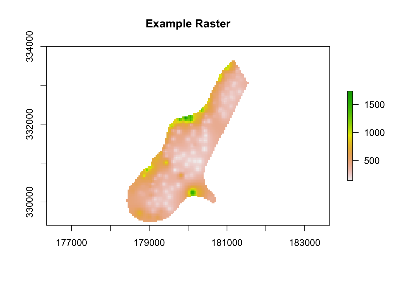

3.0.2.2.5 Types of Raster Objects

In R, there are different types of raster objects: 1. RasterLayer: A single raster layer (e.g., temperature).
2. RasterStack: A collection of multiple raster layers (e.g., temperature, precipitation, elevation).
3. RasterBrick: Similar to RasterStack, but more efficient for large datasets.

3.0.2.2.6 Trade-offs of Raster Data

Finer Resolution:
- Captures more detail (e.g., 1 m grid cells show small features).
- BUT: Increases file size and processing time.
Coarser Resolution:
- Faster processing.
- BUT: Loses fine details.

Fun Fact: Did you know satellite images, like those from NASA’s Landsat program, are raster data?

3.0.3 Key Takeaways

Vector Data	Raster Data
Points, lines, polygons	Grid of cells (pixels)
Best for discrete features	Best for continuous variables
Examples: Roads, rivers, areas	Examples: Elevation, temperature

Next, we’ll explore Coordinate Reference Systems (CRS) and learn how they ensure that spatial data aligns correctly on a map. Stay tuned! 🌐

3.0.4 3. Coordinate Reference Systems (CRS) 🌍

A Coordinate Reference System (CRS) is fundamental to working with spatial data. It ensures that data layers align properly on a map and that distances, areas, and other geographic relationships are accurately represented.

3.0.4.1 3.1. What is a CRS?

A CRS defines how locations on Earth’s surface are mapped onto a flat 2D plane. Since Earth is a 3D sphere (or an ellipsoid), CRSs are necessary for projecting this curved surface into a flat map.

Two Main Types of CRS

Angular Coordinates
- Use latitude (y) and longitude (x) to represent positions.
- Commonly used for global datasets.
- Example: WGS84 (EPSG:4326) is the standard CRS for GPS systems.
Planar Coordinates
- Transform Earth’s 3D surface into a 2D map using projections.
- Examples:
  - Mercator: Great for navigation, but distorts areas near the poles.
  - UTM (Universal Transverse Mercator): Divides the world into zones for high-accuracy mapping.
  - Albers Equal-Area: Maintains accurate area measurements, often used in environmental studies.

Did You Know?
The shape of Earth is not a perfect sphere; it’s an ellipsoid. This slight flattening at the poles affects how CRSs are designed.

3.0.4.2 3.2. Why CRS Matters

CRS is critical because spatial datasets from different sources often use different coordinate systems. If the CRSs don’t match, layers won’t align, leading to inaccurate results.

3.0.4.2.1 Key Reasons Why CRS is Important

Alignment
Ensures datasets from different sources overlap correctly on a map.
- Example: A road layer in WGS84 might not align with a satellite image in UTM until both are reprojected into the same CRS.
Accuracy
Preserves the integrity of spatial relationships like distance and area.
- Example: Calculating the area of a forest in the wrong CRS could result in significant errors.

3.0.4.2.2 Real-World Example

Incorrect CRS:

library(sf)
# Load two layers
layer1 <- st_read(system.file("shape/nc.shp", package = "sf"))
#> Reading layer `nc' from data source 
#>   `/Library/Frameworks/R.framework/Versions/4.4-arm64/Resources/library/sf/shape/nc.shp' 
#>   using driver `ESRI Shapefile'
#> Simple feature collection with 100 features and 14 fields
#> Geometry type: MULTIPOLYGON
#> Dimension:     XY
#> Bounding box:  xmin: -84.32385 ymin: 33.88199 xmax: -75.45698 ymax: 36.58965
#> Geodetic CRS:  NAD27
layer2 <- st_transform(layer1, crs = 3857)  # Transform to Web Mercator

# Plot misaligned layers
plot(st_geometry(layer1), col = "blue", main = "Misaligned Layers")
plot(st_geometry(layer2), col = "red", add = TRUE)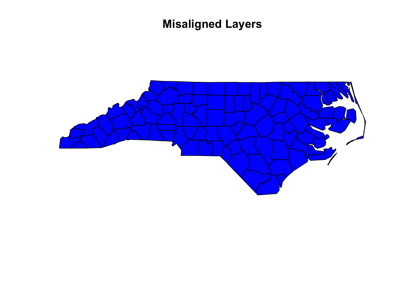

The two layers won’t overlap because they have different CRSs.

Correct CRS:

# Transform both layers to the same CRS
layer2 <- st_transform(layer2, crs = st_crs(layer1))

# Plot aligned layers
plot(st_geometry(layer1), col = "blue", main = "Aligned Layers")
plot(st_geometry(layer2), col = "red", add = TRUE)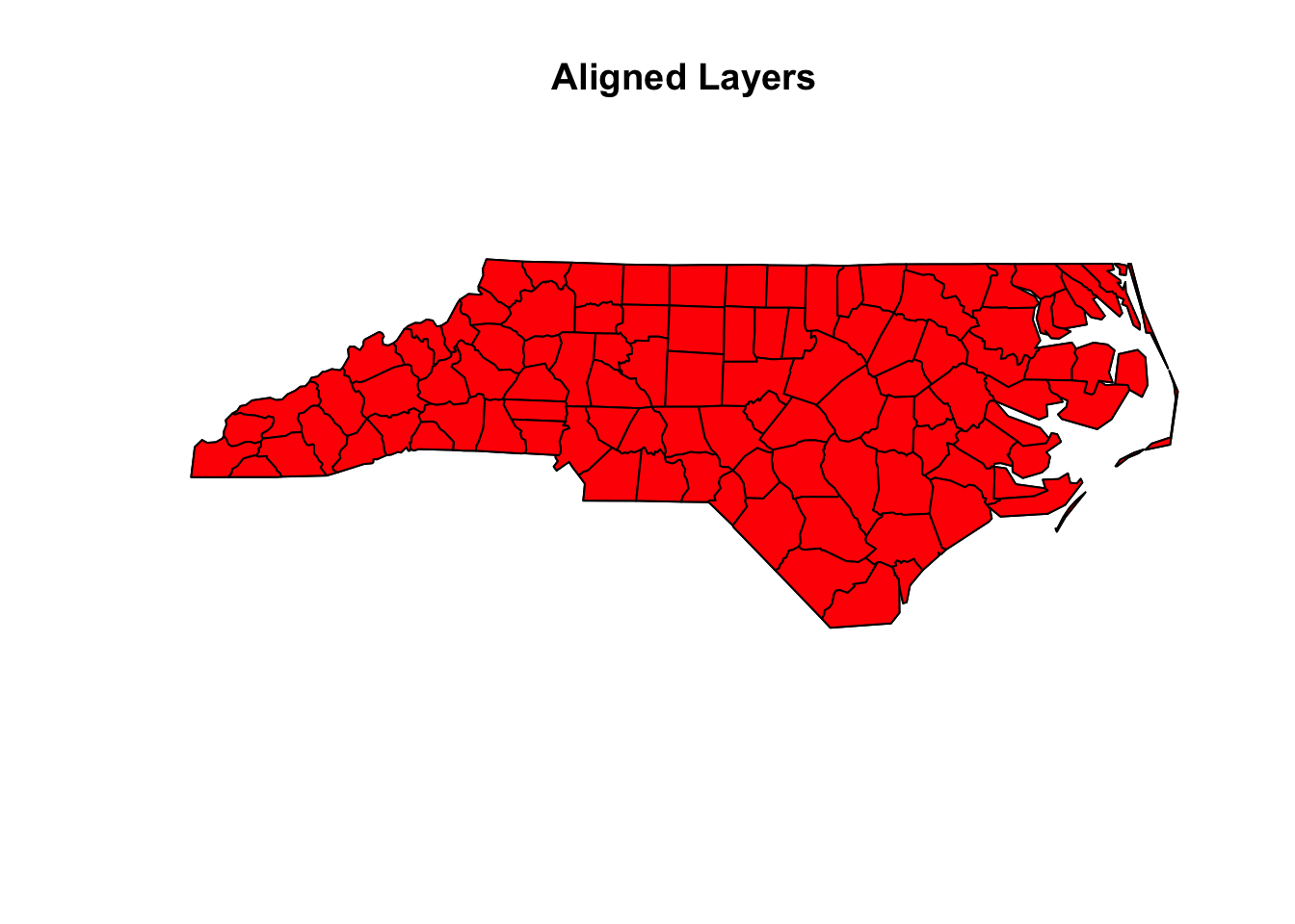

> Now the layers align perfectly.

3.0.4.3 3.3. CRS in R

R provides powerful tools to handle CRSs, primarily through the sf and terra packages.

3.0.4.3.1 Checking CRS in R

Use st_crs() to check the CRS of a vector object:

library(sf)
# Load a shapefile
nc <- st_read(system.file("shape/nc.shp", package = "sf"))
#> Reading layer `nc' from data source 
#>   `/Library/Frameworks/R.framework/Versions/4.4-arm64/Resources/library/sf/shape/nc.shp' 
#>   using driver `ESRI Shapefile'
#> Simple feature collection with 100 features and 14 fields
#> Geometry type: MULTIPOLYGON
#> Dimension:     XY
#> Bounding box:  xmin: -84.32385 ymin: 33.88199 xmax: -75.45698 ymax: 36.58965
#> Geodetic CRS:  NAD27

# Check the CRS
st_crs(nc)
#> Coordinate Reference System:
#>   User input: NAD27 
#>   wkt:
#> GEOGCRS["NAD27",
#>     DATUM["North American Datum 1927",
#>         ELLIPSOID["Clarke 1866",6378206.4,294.978698213898,
#>             LENGTHUNIT["metre",1]]],
#>     PRIMEM["Greenwich",0,
#>         ANGLEUNIT["degree",0.0174532925199433]],
#>     CS[ellipsoidal,2],
#>         AXIS["latitude",north,
#>             ORDER[1],
#>             ANGLEUNIT["degree",0.0174532925199433]],
#>         AXIS["longitude",east,
#>             ORDER[2],
#>             ANGLEUNIT["degree",0.0174532925199433]],
#>     ID["EPSG",4267]]

3.0.4.3.2 Transforming CRS in R

You can reproject (transform) a spatial object to a different CRS using st_transform():

# Transform to WGS84 (EPSG:4326)
nc_wgs84 <- st_transform(nc, crs = 4326)

# Verify the new CRS
st_crs(nc_wgs84)
#> Coordinate Reference System:
#>   User input: EPSG:4326 
#>   wkt:
#> GEOGCRS["WGS 84",
#>     ENSEMBLE["World Geodetic System 1984 ensemble",
#>         MEMBER["World Geodetic System 1984 (Transit)"],
#>         MEMBER["World Geodetic System 1984 (G730)"],
#>         MEMBER["World Geodetic System 1984 (G873)"],
#>         MEMBER["World Geodetic System 1984 (G1150)"],
#>         MEMBER["World Geodetic System 1984 (G1674)"],
#>         MEMBER["World Geodetic System 1984 (G1762)"],
#>         MEMBER["World Geodetic System 1984 (G2139)"],
#>         ELLIPSOID["WGS 84",6378137,298.257223563,
#>             LENGTHUNIT["metre",1]],
#>         ENSEMBLEACCURACY[2.0]],
#>     PRIMEM["Greenwich",0,
#>         ANGLEUNIT["degree",0.0174532925199433]],
#>     CS[ellipsoidal,2],
#>         AXIS["geodetic latitude (Lat)",north,
#>             ORDER[1],
#>             ANGLEUNIT["degree",0.0174532925199433]],
#>         AXIS["geodetic longitude (Lon)",east,
#>             ORDER[2],
#>             ANGLEUNIT["degree",0.0174532925199433]],
#>     USAGE[
#>         SCOPE["Horizontal component of 3D system."],
#>         AREA["World."],
#>         BBOX[-90,-180,90,180]],
#>     ID["EPSG",4326]]

3.0.4.3.3 Working with Raster Data

For raster data, use the crs() function from the terra or raster packages:

library(terra)
#> terra 1.8.5

# Load a raster
r <- rast(system.file("ex/elev.tif", package = "terra"))

# Check the CRS
crs(r)
#> [1] "GEOGCRS[\"WGS 84\",\n    ENSEMBLE[\"World Geodetic System 1984 ensemble\",\n        MEMBER[\"World Geodetic System 1984 (Transit)\"],\n        MEMBER[\"World Geodetic System 1984 (G730)\"],\n        MEMBER[\"World Geodetic System 1984 (G873)\"],\n        MEMBER[\"World Geodetic System 1984 (G1150)\"],\n        MEMBER[\"World Geodetic System 1984 (G1674)\"],\n        MEMBER[\"World Geodetic System 1984 (G1762)\"],\n        MEMBER[\"World Geodetic System 1984 (G2139)\"],\n        ELLIPSOID[\"WGS 84\",6378137,298.257223563,\n            LENGTHUNIT[\"metre\",1]],\n        ENSEMBLEACCURACY[2.0]],\n    PRIMEM[\"Greenwich\",0,\n        ANGLEUNIT[\"degree\",0.0174532925199433]],\n    CS[ellipsoidal,2],\n        AXIS[\"geodetic latitude (Lat)\",north,\n            ORDER[1],\n            ANGLEUNIT[\"degree\",0.0174532925199433]],\n        AXIS[\"geodetic longitude (Lon)\",east,\n            ORDER[2],\n            ANGLEUNIT[\"degree\",0.0174532925199433]],\n    USAGE[\n        SCOPE[\"Horizontal component of 3D system.\"],\n        AREA[\"World.\"],\n        BBOX[-90,-180,90,180]],\n    ID[\"EPSG\",4326]]"

# Transform CRS
r_transformed <- project(r, "+proj=utm +zone=33 +datum=WGS84 +units=m")

3.0.4.4 3.4. Common CRS Notations

PROJ.4 Strings:
Text-based format describing CRS properties. Example:
```
+proj=utm +zone=33 +datum=WGS84 +units=m +no_defs
```
EPSG Codes:
Numeric identifiers for CRSs. Examples:
- EPSG:4326: WGS84, the most commonly used CRS.
- EPSG:3857: Web Mercator, used by Google Maps.

3.0.4.5 Key Takeaways

Task	Function	Package
Check CRS	`st_crs()`	`sf`
Transform CRS	`st_transform()`	`sf`
Check CRS (Raster)	`crs()`	`terra`
Set or Transform CRS	`project()`	`terra`

Reminder: Always ensure your spatial layers have the same CRS before performing any analysis.

By mastering CRS concepts and tools, you’ll avoid alignment errors and ensure accurate spatial analysis. In the next section, we’ll dive into spatial data tools in R! 🚀

3.0.5 4. Spatial Data Tools in R 🛠️

In this section, we’ll explore the key tools and functions in R for working with spatial data. These tools allow us to load, manipulate, and visualize both vector and raster data.

3.0.5.1 4.1. Vector Data Tools ✏️

Vector data consists of points, lines, and polygons that represent discrete features on a map (e.g., cities, rivers, and country boundaries).

3.0.5.1.1 Key Functions for Vector Data

st_read():
Loads vector data from various file formats (e.g., shapefiles, GeoJSON).

   library(sf)
   # Load a shapefile of North Carolina counties
   nc <- st_read(system.file("shape/nc.shp", package = "sf"))
#> Reading layer `nc' from data source 
#>   `/Library/Frameworks/R.framework/Versions/4.4-arm64/Resources/library/sf/shape/nc.shp' 
#>   using driver `ESRI Shapefile'
#> Simple feature collection with 100 features and 14 fields
#> Geometry type: MULTIPOLYGON
#> Dimension:     XY
#> Bounding box:  xmin: -84.32385 ymin: 33.88199 xmax: -75.45698 ymax: 36.58965
#> Geodetic CRS:  NAD27

plot():
Visualizes vector data.

# Plot the shapefile
plot(nc["NAME"], main = "Counties in North Carolina")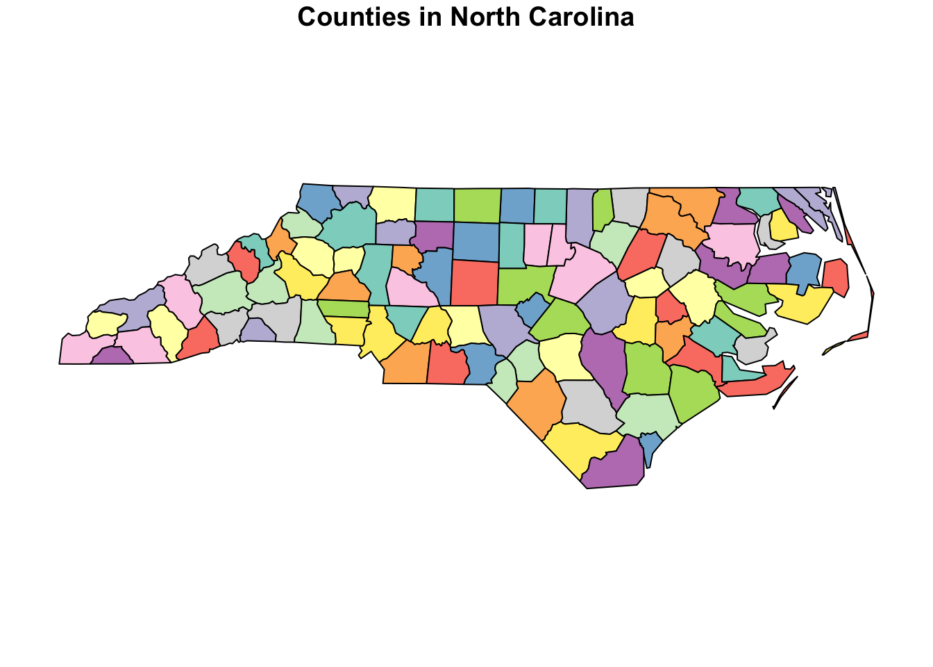

st_transform():
Reprojects vector data to a different CRS.

# Transform to WGS84
nc_wgs84 <- st_transform(nc, crs = 4326)

st_write():
Saves vector data to a file (e.g., shapefile or GeoJSON).

st_write(nc, "nc_counties.geojson", append=TRUE)

3.0.5.1.2 Common File Formats for Vector Data

Format	Description
Shapefile (.shp)	A widely used format for vector data, but requires multiple associated files (.shp, .shx, .dbf).
GeoJSON	A lightweight, text-based format for vector data, often used in web mapping applications.
KML	Used by Google Earth to represent geographic data.

Did You Know?
The shapefile format was introduced by Esri in the early 1990s and remains one of the most commonly used vector data formats, despite its limitations.

3.0.5.2 4.2. Raster Data Tools 🌄

Raster data represents the world as a grid of cells, where each cell has a value (e.g., elevation, temperature).

3.0.5.2.1 Key Functions for Raster Data

raster():
Loads raster data from a file.

library(raster)
# Load a sample raster
r <- raster(system.file("external/test.grd", package = "raster"))

terra::rast():
An alternative to raster() from the terra package, which offers better performance.

library(terra)
# Load the raster using terra but from raster's sample file
# in your local machine, run this commented line:
#r_terra <- rast(system.file("external/test.grd", package = "raster"))
# for demonstration, we do this:
r_terra = rast("datasets/sample_raster.tif")
plot(r_terra, main = "Sample Raster Loaded with terra")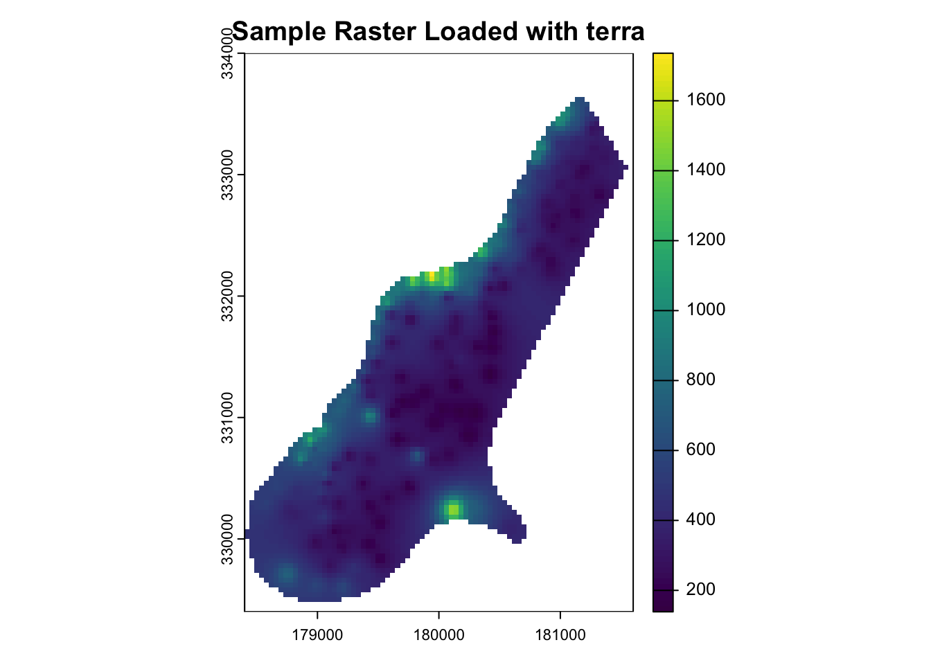

plot():
Visualizes raster layers.

# Plot the raster
plot(r, main = "Example Raster Layer")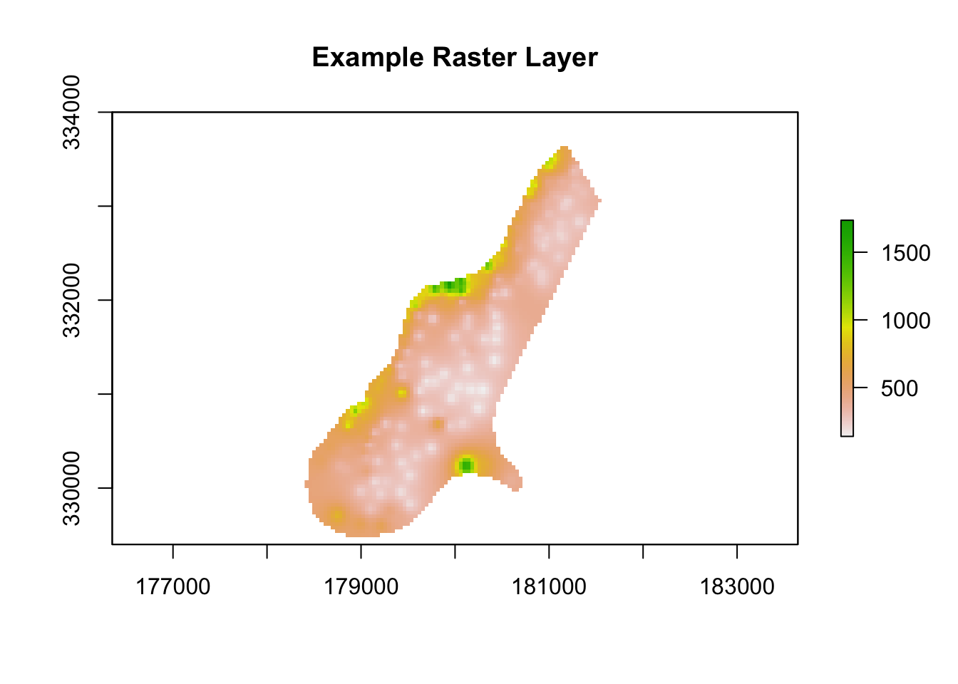

writeRaster():
Saves raster data to a file (e.g., GeoTIFF).

# Save the raster as a GeoTIFF file
writeRaster(r, "example_raster.tif", format = "GTiff", overwrite=TRUE)

3.0.5.2.2 Common File Formats for Raster Data

Format	Description
GeoTIFF	High-resolution raster format that supports metadata.
NetCDF	Commonly used for climate and environmental data, supports multi-dimensional data.
ASCII Grid	A text-based format for raster data, but less efficient than GeoTIFF.
GRIB	Widely used for weather data, stores compressed raster data.

Fun Fact:
GeoTIFF is a georeferenced version of the popular TIFF image format. It’s widely used in remote sensing and GIS applications because it stores spatial information alongside the image data.

3.0.5.3 Key Differences Between Vector and Raster Tools

Aspect	Vector Tools (`sf`, `terra`)	Raster Tools (`raster`, `terra`)
Data Representation	Points, lines, and polygons	Grid of cells (pixels)
Common Functions	`st_read()`, `st_transform()`, `st_write()`	`raster()`, `plot()`, `writeRaster()`
Common File Formats	Shapefiles, GeoJSON, KML	GeoTIFF, NetCDF, ASCII Grid

3.0.5.4 Practical Example: Combining Vector and Raster Data

Let’s say we want to extract the elevation values at specific observation points (vector data) from a digital elevation model (raster data):

library(sf)
library(raster)

# Load vector data (polygons)
nc <- st_read(system.file("shape/nc.shp", package = "sf"))
#> Reading layer `nc' from data source 
#>   `/Library/Frameworks/R.framework/Versions/4.4-arm64/Resources/library/sf/shape/nc.shp' 
#>   using driver `ESRI Shapefile'
#> Simple feature collection with 100 features and 14 fields
#> Geometry type: MULTIPOLYGON
#> Dimension:     XY
#> Bounding box:  xmin: -84.32385 ymin: 33.88199 xmax: -75.45698 ymax: 36.58965
#> Geodetic CRS:  NAD27

# Load the saved raster file
elev <- raster("datasets/elevation_data.grd")

# Calculate centroids of the polygons
centroids <- st_centroid(nc)
#> Warning: st_centroid assumes attributes are constant over
#> geometries

# Extract only the X and Y coordinates of the centroids
coords <- st_coordinates(centroids)

# Extract elevation values at the centroids
elevation_values <- extract(elev, coords)

# Add extracted values as a new column
nc$elevation <- elevation_values

# View the updated data
head(nc)
#> Simple feature collection with 6 features and 15 fields
#> Geometry type: MULTIPOLYGON
#> Dimension:     XY
#> Bounding box:  xmin: -81.74107 ymin: 36.07282 xmax: -75.77316 ymax: 36.58965
#> Geodetic CRS:  NAD27
#>    AREA PERIMETER CNTY_ CNTY_ID        NAME  FIPS FIPSNO
#> 1 0.114     1.442  1825    1825        Ashe 37009  37009
#> 2 0.061     1.231  1827    1827   Alleghany 37005  37005
#> 3 0.143     1.630  1828    1828       Surry 37171  37171
#> 4 0.070     2.968  1831    1831   Currituck 37053  37053
#> 5 0.153     2.206  1832    1832 Northampton 37131  37131
#> 6 0.097     1.670  1833    1833    Hertford 37091  37091
#>   CRESS_ID BIR74 SID74 NWBIR74 BIR79 SID79 NWBIR79
#> 1        5  1091     1      10  1364     0      19
#> 2        3   487     0      10   542     3      12
#> 3       86  3188     5     208  3616     6     260
#> 4       27   508     1     123   830     2     145
#> 5       66  1421     9    1066  1606     3    1197
#> 6       46  1452     7     954  1838     5    1237
#>                         geometry elevation
#> 1 MULTIPOLYGON (((-81.47276 3...        NA
#> 2 MULTIPOLYGON (((-81.23989 3...        NA
#> 3 MULTIPOLYGON (((-80.45634 3...        NA
#> 4 MULTIPOLYGON (((-76.00897 3...        NA
#> 5 MULTIPOLYGON (((-77.21767 3...        NA
#> 6 MULTIPOLYGON (((-76.74506 3...        NA

Tip:
Use the terra package for faster processing when working with large raster datasets.

By mastering these tools, you’ll be well-equipped to handle a wide range of spatial data tasks in R. Next, we’ll explore spatial analysis techniques, including buffering, overlay operations, and spatial joins! 🚀

3.0.6 5. Practical Considerations 🛠️

Working with spatial data requires careful attention to detail to ensure accurate analysis and meaningful results. Let’s go over some important practical considerations when using spatial data.

3.0.6.1 5.1. Data Alignment

When combining different spatial datasets, it’s crucial to ensure they are properly aligned. Misaligned data can lead to incorrect analysis and misleading results.

Key Points for Data Alignment:

Same CRS
- All spatial layers (vector and raster) should use the same Coordinate Reference System (CRS).
- Example: If your vector data uses EPSG:4326 (WGS84), your raster data should be reprojected to match this CRS.

library(sf)
library(terra)
 
# Load vector data
nc <- st_read(system.file("shape/nc.shp", package = "sf"))
#> Reading layer `nc' from data source 
#>   `/Library/Frameworks/R.framework/Versions/4.4-arm64/Resources/library/sf/shape/nc.shp' 
#>   using driver `ESRI Shapefile'
#> Simple feature collection with 100 features and 14 fields
#> Geometry type: MULTIPOLYGON
#> Dimension:     XY
#> Bounding box:  xmin: -84.32385 ymin: 33.88199 xmax: -75.45698 ymax: 36.58965
#> Geodetic CRS:  NAD27

# Load raster data
elev <- rast("datasets/elevation_data.grd")
   
# Check CRS of both datasets
st_crs(nc)  # Vector CRS
#> Coordinate Reference System:
#>   User input: NAD27 
#>   wkt:
#> GEOGCRS["NAD27",
#>     DATUM["North American Datum 1927",
#>         ELLIPSOID["Clarke 1866",6378206.4,294.978698213898,
#>             LENGTHUNIT["metre",1]]],
#>     PRIMEM["Greenwich",0,
#>         ANGLEUNIT["degree",0.0174532925199433]],
#>     CS[ellipsoidal,2],
#>         AXIS["latitude",north,
#>             ORDER[1],
#>             ANGLEUNIT["degree",0.0174532925199433]],
#>         AXIS["longitude",east,
#>             ORDER[2],
#>             ANGLEUNIT["degree",0.0174532925199433]],
#>     ID["EPSG",4267]]
crs(elev)   # Raster CRS
#> [1] "PROJCRS[\"unknown\",\n    BASEGEOGCRS[\"unknown\",\n        DATUM[\"World Geodetic System 1984\",\n            ELLIPSOID[\"WGS 84\",6378137,298.257223563,\n                LENGTHUNIT[\"metre\",1]],\n            ID[\"EPSG\",6326]],\n        PRIMEM[\"Greenwich\",0,\n            ANGLEUNIT[\"degree\",0.0174532925199433],\n            ID[\"EPSG\",8901]]],\n    CONVERSION[\"unknown\",\n        METHOD[\"Oblique Stereographic\",\n            ID[\"EPSG\",9809]],\n        PARAMETER[\"Latitude of natural origin\",52.1561605555556,\n            ANGLEUNIT[\"degree\",0.0174532925199433],\n            ID[\"EPSG\",8801]],\n        PARAMETER[\"Longitude of natural origin\",5.38763888888889,\n            ANGLEUNIT[\"degree\",0.0174532925199433],\n            ID[\"EPSG\",8802]],\n        PARAMETER[\"Scale factor at natural origin\",0.9999079,\n            SCALEUNIT[\"unity\",1],\n            ID[\"EPSG\",8805]],\n        PARAMETER[\"False easting\",155000,\n            LENGTHUNIT[\"metre\",1],\n            ID[\"EPSG\",8806]],\n        PARAMETER[\"False northing\",463000,\n            LENGTHUNIT[\"metre\",1],\n            ID[\"EPSG\",8807]]],\n    CS[Cartesian,2],\n        AXIS[\"(E)\",east,\n            ORDER[1],\n            LENGTHUNIT[\"metre\",1,\n                ID[\"EPSG\",9001]]],\n        AXIS[\"(N)\",north,\n            ORDER[2],\n            LENGTHUNIT[\"metre\",1,\n                ID[\"EPSG\",9001]]]]"
   
# Reproject vector data to match raster CRS
nc_aligned <- st_transform(nc, crs(elev))

Align Raster Layers
- When working with multiple raster layers (e.g., temperature, precipitation), ensure they have the same resolution, extent, and origin.
- This ensures they can be used together without errors in analysis.

3.0.6.2 5.2. Data Quality

Always check your data for missing values or inconsistencies before analysis. Poor data quality leads to unreliable models.

Steps to Ensure Data Quality:

Check for Missing Values
- Raster data often contains cells with NoData values.
- You can use terra to check and handle these missing values:

# Check for NoData cells
summary(elev)
#>       test       
#>  Min.   : 138.7  
#>  1st Qu.: 294.0  
#>  Median : 371.9  
#>  Mean   : 425.6  
#>  3rd Qu.: 501.0  
#>  Max.   :1736.1  
#>  NA's   :6022

# Replace NoData cells with 0 (if appropriate)
elev[is.na(elev)] <- 0
summary(elev)
#>       test       
#>  Min.   :   0.0  
#>  1st Qu.:   0.0  
#>  Median :   0.0  
#>  Mean   : 147.0  
#>  3rd Qu.: 302.8  
#>  Max.   :1736.1

We observe now that there are no missing observations in the data.

Remove Duplicates in Vector Data
- If your vector data contains duplicate points, it can bias your analysis.
- Use distinct() from dplyr or st_as_sf() to remove duplicates:

library(dplyr)
#> 
#> Attaching package: 'dplyr'
#> The following objects are masked from 'package:terra':
#> 
#>     intersect, union
#> The following objects are masked from 'package:raster':
#> 
#>     intersect, select, union
#> The following objects are masked from 'package:stats':
#> 
#>     filter, lag
#> The following objects are masked from 'package:base':
#> 
#>     intersect, setdiff, setequal, union
nc <- distinct(nc)

3.0.6.3 5.3. Computational Trade-offs

High-resolution data provides more detail but increases computation time and memory usage. Choose a resolution appropriate for your study area.

Key Considerations:

Resolution
- High-resolution data (e.g., 1 m cells) is great for detailed analysis but requires significant computational power.
- Low-resolution data (e.g., 10 km cells) is faster to process but may miss important details.
Tip: Start with lower resolution data when prototyping your analysis, then switch to high-resolution data for the final results.
Extent
- Limiting the spatial extent of your data can reduce processing time. If you’re only interested in a specific region, crop your raster to that region:
```
# Crop raster to the extent of vector data
elev_cropped <- crop(elev, st_bbox(nc))
```

3.0.7 6. Fun Facts and Tips 🎉

Did You Know?
- Raster data is like an image grid, where each pixel stores environmental information, such as temperature or elevation.
Pro Tip:
- Use the terra package instead of raster for faster computations with large datasets. It’s designed to handle big spatial data more efficiently.
Fun Fact:
- The Mercator projection distorts areas near the poles, which is why Greenland looks much larger than it actually is!

3.0.8 7. Summary and Key Takeaways 📝

Let’s wrap up what we’ve learned:

Spatial Data Types
- Vector data: Points, lines, polygons.
- Raster data: Grids of cells with values representing continuous data.
CRS Importance
- Always ensure that your spatial datasets have the same CRS to avoid alignment issues.
- Use functions like st_transform() (vector) and project() (raster) to reproject data when needed.
R Packages for Spatial Data
- Use sf for vector data and terra for raster data.
- These packages provide modern, efficient workflows for handling spatial data in R.

With these concepts in mind, you’re well on your way to becoming proficient in handling spatial data in R! Next, we’ll explore more advanced topics, such as spatial analysis techniques and model building. Stay tuned! 🚀

2 Introduction

4 Spartial Data in R